The Element Protocol Construction Paper

Note: This paper is not final, hence the title “construction paper” and will be updated over time. The opinions and analysis reflected herein are subject to change or updates over time.
Contents
- 1.Introduction
- 2. Principal Tokens
- 3. Yield Tokens
- 4. Minting and Providing Liquidity
- 5. Market Forces
- 6. Building on top of the Element Protocol
- 7. Summary
- 8. Appendix
1. Introduction
1.1 Overview
Element Finance is a protocol which enables users to seek high fixed yield income in the DeFi market, initially focused on ETH, BTC, USDC, and DAI. Users can access, via the ecosystem and existing AMMs, ETH, BTC, USDC, and DAI at a discount without being locked into a term, allowing the exchange of the discounted asset and the base asset at any time. The fixed rate income can be secured with the exchange of any major base asset. For active DeFi users, the Element Protocol enables capital efficiency on yield positions they are already depositing into, such as Yearn or ETH2 staking. Users can sell their deposited principal at a discount as fixed yield income, leveraging or increasing exposure to yield without liquidation risk. This competitive activity is what drives the high fixed yield markets. This construction paper breaks down the Element Protocol and discusses how it can open the door to a number of new primitives and innovations. When users sell their principal or yield, risk is not transferred to another asset. The assets are redeemable for the underlying position directly and denominated in the original position.
1.2 The Current State of Yield Markets in DeFi
Today, in the decentralized finance (DeFi) space, the variable yield market can be both difficult and overwhelming for casual users to navigate. Yield rates constantly fluctuate, resulting in users needing to move their funds regularly in order to meet their target APY, and depositing or shifting between positions regularly incurs high transaction fees.
Securing fixed rate yield can resolve these issues. However, the current fixed rate yield products on the market offer low rates and do not have enough liquidity to enter in and out of the position easily. This lack of liquidity causes slippage problems or the inability to exit from a position until after a defined term. In other cases, depositing into a fixed rate position requires multiple transactions and the associated high transaction fees that come with it.
Capital efficiency is an underserved feature for DeFi users. When users are required to have their principal locked in a yield generating position, such as a Yearn vault or ETH2 staking, they cannot access further opportunities, incur significant costs if they decide to move their position, and the market often lacks liquidity.
1.3 The Element Approach
The Element Protocol, at its core, works by enabling users via the Ethereum contracts to split the base asset (ETH, BTC, USDC, DAI) of yield generating positions, such as a Yearn vault or an ETH2 validator, into two separate, fungible tokens: the Principal Token (PT), and the Yield Token (YT).
The splitting mechanism allows users to sell their principal at a discount, thus giving users the ability to create a marketplace for fixed rate income positions. Their principal is no longer locked up and they may use their newly freed funds to leverage at high multiples, gaining increased exposure to yield without the typical liquidation risk. Users may also gain additional trading fees or APY on their yield positions by using their new tokens to provide liquidity into an AMM. The casual user subsidizes the DeFi user’s active strategies by securing fixed rate yield at a discount on what the DeFi user earns. The DeFi user’s participation subsidizes the value of the fixed rate yield.
Element's approach takes an alternative approach to tranching products, instead enabling users in the market to set the price of fixed vs. variable yield rates. This competitive activity along with the custom curve built on Balancer V2 to support the PTs is what drives the high fixed yield markets. Furthermore, it promotes liquidity in the fixed yield income market while minimizing slippage, fees, and impermanent loss, ultimately opening the door to a number of new DeFi primitives.
1.4 Glossary Definitions
- Principal Tokens (PTs): The token representing the user's deposit value into the Element Protocol. These tokens are redeemable 1-for-1 for the underlying asset at maturity.
- Yield Tokens (YTs): The token representing the variable yield gain over the term period for the deposited underlying asset.
- Principal Reserves: The number of PTs staked in a pool pairing of the base asset and the PT. For example, the number of eP:yETH staked in the pool pairing of ETH/eP:yETH.
- Base Asset: The asset deposited into the Element Protocol (BTC, ETH, USDC, or DAI).
- Base Asset Reserves: The number of base assets staked in a pool pairing of the base asset with the PTs of said base asset. For example, the number of ETH staked in the pool pairing of ETH/eP:yETH.
- Time Stretch Parameter: A parameter used in the trading curve that affects the price discoverability, fees, and liquidity provision ratio of the base asset to PTs.
- Annual Percentage Yield (APY): Annual Percentage Yield is a time-based measurement of the Return On Investment (ROI) on an asset.
- For example, $100 invested at 5% APY would yield $105 after one year, if there is no compounding of any yield earned on that $100 through the year. Assuming a static APY rate, the Monthly ROI would be 0.41%.
- Target APY: The User's targeted Annual Percentage Yield.
- Term: A duration of time in which a user's assets are generating yield and deposited in the Element Protocol.
- Term length: The duration in which the user chooses to have their asset deposited in the Element Protocol, generating yield.
- Vault: A generic term for a yield-bearing asset.
- yVault: A programmatically adjusted lending aggregator, arbitrageur, and optimized yield generator (reference).
- Automated Market Maker (AMM): An AMM is a system that provides liquidity to the exchange it operates in through automated trading.
- LP tokens: Tokens representing a user's liquidity position in an AMM.
- Impermanent Loss (IL): A loss that occurs when the value of the deposit asset is less compared to when they were deposited. In short, Impermanent loss is the difference between holding tokens in an AMM and holding them in your wallet. It occurs when the price of the tokens inside an AMM diverges in any direction. The more divergence, the greater the impermanent loss.
- Slippage: The amount the price moves in a trading pair between when a transaction is submitted and when it is executed.
- Yield Token Compounding: Depositing in a yield position and selling the principal to re-deposit, increasing exposure to yield. This is done multiple times, selling and re-depositing, and allows for leveraging into the yield at many multiples of the initial capital.
2. Principal Tokens
A Principal Token (PT) offers an asset such as BTC, ETH, USDC, or DAI that is locked for a fixed term. At the end of the term, it can be redeemed for its full value.

Figure 1
For example, if 10 ETH is used to purchase discounted ETH at a 10% APY for a one-year lockup, 11 eP:ETH or PTs will be issued. Upon expiry of the fixed term, one year later, the 11 eP:ETH is redeemable for 11 ETH. A fixed rate of yield was secured.
The locked ETH will always be worth less than readily available ETH. Readily available ETH can be staked in a yield position, gaining active yield. For this lost opportunity, these PTs or locked ETH will be priced at a discount, likely relative to the current yield rates in the market. Purchasing this discounted ETH is akin to securing a fixed rate yield. At the time of purchase, the discount and yield are already known.
As a further example, if the current rate for providing liquidity for ETH is 15% annualized variable yield, a user may sell the PTs at a slightly lower rate. This gives a guaranteed stable yield rate to the purchaser and prevents them from having to shift their assets between DeFi protocols in the situation where the variable yield decreases. Additionally, it allows users to avoid costly transaction fees and other inconvenient complexities.
Although the terminology "locked" is used to describe the process of entering a fixed yield position, it is important to note that the Element Protocol is designed to optimize for liquidity allowing users to exit their position at any time, while still enabling users to gain yield until they decide to exit.
Note: The use of 1-year terms in the examples of this paper is purely for simplicity. The Element protocol will initially allow users to mint both 6-month and 3-month terms.
2.1. Initial Use Cases of Principal Tokens
Purchasing PTs can provide a wide variety of utility depending on a user's market strategy. This section provides an in-depth look into some of those utilities. Additionally, Section 5 of this paper covers the possible use cases surrounding the minting and selling of PTs in an active market.
Yield, Fixed Yield, and Stability
In today's market, the current variable yield positions available fluctuate constantly, frequently changing day-to-day. In a single week, a variable position that may have carried 20% APY on Tuesday may only carry 5% on Thursday. This constant fluctuation forces current DeFi users to constantly monitor the market and move their capital to different yield positions in order to maintain their desired APY.
Casual users or institutions managing large amounts of capital may not have the bandwidth or the understanding of the space and its associated risks to constantly manage and monitor their capital. Additionally, these users may not want to deal with the complexities surrounding taxes or the risks associated with new protocols being released. For these users, securing a fixed rate of income is both helpful and more appealing, allowing them to not have to actively manage their positions.
AMM Liquidity Provision
If a user is already looking to gain exposure to BTC or ETH for a period of time, it makes sense to gain that exposure at a discount. During the period of holding the discounted ETH, the user may provide liquidity for the PTs on an AMM, gaining a significant boost on their fixed rate yield via trading fees. The mechanism behind providing liquidity for PTs and their profitability is described in further detail in Section 4.
Bearish on Variable Yield
A DeFi user may believe that the current yield rates offered in the market are high and suspects that rates will begin to decrease over the next 3-6 months. As a result, the user decides to secure a high fixed rate yield and thus, hedges against a yield downturn in the market.
Principal Tokens as a Trading Instrument
From the perspective of a swing trader who enters positions ranging from periods of 1-2 weeks up to a calendar month, PTs make for a better form of trading instrument generating a higher rate of return without incurring added trading risks.
Spot Trading
Assuming the following parameters:
- Annual Fixed Rate Yield*: 10%
- Asset Being Swing Traded*: 1 Month, ptBTC
- Current Price of BTC*: $50,000
- Price Target of BTC in Trade*: $55,000
- Trade Duration*: 1 Month
- USD Amount in Trade*: $200,000
A spot trader, Anna, may choose to take a trading position between 2 to 4 weeks. Her analysis leads her to believe that BTC will increase in value by 10% at the end of the calendar month. She made the right call and hits her price target of $55,000, redeeming her PT for 4.033 BTC at a price of $55,000 per BTC.
In concluding the trade, her total assets sum up to $221,815. If she had taken a BTC position instead of an eP:BTC position, her total asset sum would be a total of $220,000. By using PTs as her primary trading instrument, she gained an additional component of profitability in the form of fixed yield on top of her typical trading profits.
2.2 Future Use Cases of Principal Tokens
After the Element protocol has been released, a number of future structured products can be built by third parties on top of its foundation which may further drive demand for purchasing PTs. Section 6 provides an in-depth look at some of the potential structured products that could be built on top of the Element Protocol:
- 1:1 Collateralized Loans
- Fixed Term Lending
- Yield Ladders
3. Yield Tokens
The redemption value for a YT at the end of the defined term will be the average yield it has earned over the course of the term on the principal it represents.
Example:
- eY:yETH represents the yield gained on an ETH Yearn position listed at 25% APY.
- 1 eY:yETH reflects the yield gained from 1 ETH principal.
- The eY:yETH is under a 1-year term.
- If the Yearn position maintains 25% APY for the entire year, eY:yETH is redeemable for 0.25 ETH.

Figure 2
However, by definition, no variable yield position on the market maintains its listed yield rate (APY). The APYs constantly fluctuate. This implies that the real redeemable yield at the end of the year is unknown.
The combined yield token and principal token redemption at maturity will not exceed the value of the yield asset in the Ethereum contracts. The yield token is only redeemable for the differential in value of the underlying yield asset from the original principal. It does not transfer financial risk associated with a future change in any such value or level without also conveying a current or future direct or indirect ownership interest in an asset (including any enterprise or investment pool) or liability that incorporates the financial risk so transferred. All growth or changes are denominated in the original asset.
3.1 Yield Token Pricing
How would a YT be priced? This is an extremely difficult question to answer. In an ideal world, YTs would be priced at the market's speculated average APY with an added opportunity discount.
For example, if the market speculates that the yETH position would hold an average of 15% APY over the next year, the assumed redemption price of 1 eY:yETH would be equal to 0.15 ETH. As discussed in the PTs Section, the locked 0.15 ETH will sell at a discount, however, the discount on the eY:yETH would likely be higher than simply the opportunity lost due to the intrinsic risk of speculating its average yield. There is no way of knowing what this average yield will end up truly being. It could be less than 0.15 ETH.
However, this pricing structure is naive. Other forces will impact the price. This paper will cover these details but not yet, as a better understanding of the protocol is needed first. To read about the details of the market forces that could impact the price of a YT, reference Sections 5 and 6.
Element does not in any way determine the pricing of yield tokens in the market. Users who choose to sell or buy their yield tokens on decentralized exchanges adjust the price based on automated market making curves. Any user enacting in a trade should be aware of how the curves operate. Additionally, the underlying trading vehicles or AMMs are not owned or property of Element.
3.2 Buying and Selling Opportunities for Yield Tokens
YTs can be used as a way to buy or sell the yield rate of a position.
A sophisticated DeFi user may evaluate the market’s pricing of a YT and consider it to be too aggressive or even conservative. For example, in a one-year term, the user believes the yETH vault will have an average APY of 10%. This would imply that the user thinks 1 eY:yETH will be redeemable for 0.1 ETH at the end of the term. If the YT is selling for more than a 10% discount on 0.1 ETH, then it would be considered a strong buy. In this case, the user would be taking a buy position on the YT. If it is less, then it would be considered a strong sell. In this case, the user would want to sell the YT.
4. Minting and Providing Liquidity
Minting and providing liquidity for PTs and YTs may be a very profitable endeavor for DeFi users. This section begins by covering how the minting process works and ends with a detailed look at the simulations and analysis of the potential profitability as well the liquidity providing process, such as how the trading curve and parameterization are used.
4.1 Terms
A term indicates the redemption date of a set of PTs or YTs. The principal or yield cannot be redeemed through the Element Protocol's contracts until the term date has been reached.
Although the Element Protocol smart contracts allow for any term to be created, it is expected that users and openly available frontends will encourage certain term conventions in order to concentrate liquidity. For example, users may collectively decide to actively support both 3 and 6-month terms released every month and a half. The contracts are open for anyone to integrate or launch a term with. This means the community of users will ultimately decide which terms they would like to support. This could be through a DAO or through other products that are built.
Terms are indicated by the token name and are marked with a date stamp. For example:
eY:yETH:03-Jan-2021-GMT
4.2 Minting in Depth
When minting, a user must first choose the backing collateral and the specific term to mint into. Element's initial positions will be collateralized by Yearn Vaults. The token naming conventions are reflected in the parameters. For example:
- Principal Token:
eP:yETH:03-JAN-2021-GMT - Yield Token:
eY:yETH:03-JAN-2021-GMT
The e represents Element, while the P and Y indicate whether it is a principal or yield token. The second part indicates the backing collateral, such as a Yearn ETH vault, yETH. The third and final part indicates the term or redemption date in GMT or UTC+0 time. It's important to note that tokens with identical names are fungible with each other and can be staked or traded together in an AMM.
For example, today is 01/01/2021. Minting into a term with a 3-month expiration date (04/01/2021), collateralized by the Yearn wBTC vault, produces the following tokens:
- Principal Token:
eP:ywBTC:01-APR-2021-GMT - Yield Token:
eY:ywBTC:01-APR-2021-GMT
A token with a different date or any sort of modification would not be fungible. For example, the following PT would not be fungible with the example token above since it has a different date:
- Principal Token:
eP:ywBTC:02-APR-2021-GMT
Minting Retroactively
One area of complexity that the Element Protocol handles is with the action of minting into an existing term. YTs accumulate value over time, essentially introducing their own principal. To give a simple example, if Yearn compounds daily, the YT's accumulated value looks as follows:
| Input | Minted Asset |
|---|---|
| 1 BTC | 1 eY:ywBTC |
| Day | Average APY | Total Accumulated |
|---|---|---|
| 0 | 8% | 0.000219178 |
| 1 | 7% | 0.000411001 |
| 2 | 6% | 0.000575452 |
| 3 | 9% | 0.000822169 |
| 4 | 5% | 0.000959268 |
| 5 | 10% | 0.0012335 |
| 6 | 8% | 0.00145295 |
Table 1
As displayed in the above table, once day 6 has been reached, the YT has accumulated its own principal of 0.00145 BTC.
Why does this introduce complexity? In order to mint into a term that has already compounded yield, the minter must supply that accumulated yield, otherwise, the YTs would not be fungible with each other. They would have a different market value.
The Element Protocol is optimized for users accumulating YTs, and therefore reduces the balance of the user's principal in order to cover the accumulated yield when minting. In this example, if a user chooses to mint on day 6, then 0.00145 BTC must be accounted for. As a result, 0.00145 fewer PTs are issued. The user's minted tokens would look as follows:
| Input | Minted Asset |
|---|---|
| 1 BTC | 1 eY:ywBTC |
User Balance:
- 0.99855
eP:ywBTC:01-MAR-2021-GMT - 1
eY:ywBTC:01-MAR-2021-GMT
4.3 Providing Liquidity for Principal Tokens
If a user is already depositing into Yearn, they can boost their APY even further by minting PTs and YTs. After minting both the PTs and YTs, the user may provide liquidity to the market on fixed rate or variable yield. The user now earns additional APY via trading fees from the AMM.
LP Profitability Analysis
Although future trading volume and liquidity are difficult to predict, the following analysis attempts to simulate the different scenarios. Due to market forces such as Yield Token Compounding, covered in a later section (5.2), it is predicted that trading activity may be high. These simulations predict purchasing activity to decline as the maturity period of the term comes closer. However, this prediction may not be correct, since Yield Token Compounding (discussed in Section 5) and other market activities increase profit as the maturity period comes to an end. In the scenario where the maturity period is converging, purchasing activity could also be automated via vaults or tools such as Yearn. However, with these assumptions in mind, the simulation results of a \(log(\frac{1}{term\_length})\) show a spike in activity at the beginning of a term and then decay.
The following represents a yCRVSTETH position, at 20% APY, with PTs trading at 10%:
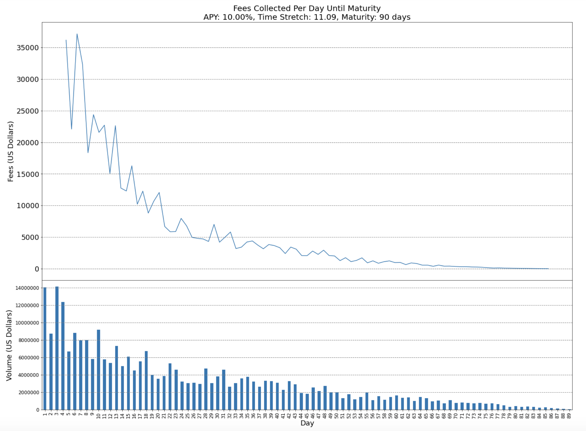
Figure 3
Order sizes are distributed as follows:
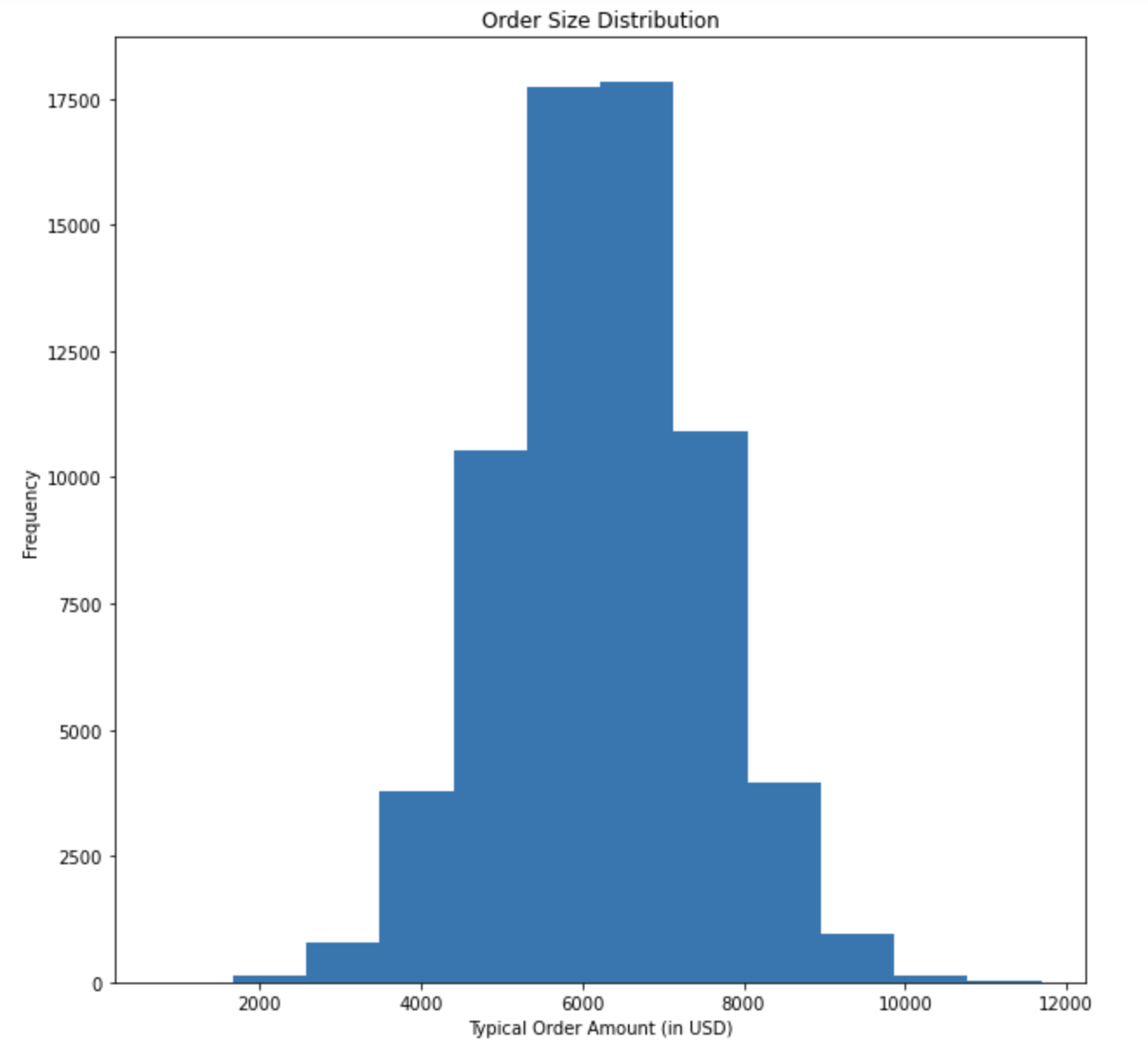
Figure 4
The following table shows the various scenarios at different trading volumes. The final column shows the resulting output APR.
| target_liquidity | trade_volume_sum | mean_daily_volume | apr |
|---|---|---|---|
| 10,000,000 | 140,113,083 | 1,556,812 | 11.76 |
| 10,000,000 | 276,382,190 | 3,070,913 | 20.34 |
Table 2
If these target volumes are maintained, providing liquidity in a 20% APY position on yCRVSTETH or a 10% PT purchase may boost to 11.76-20.34% APY, depending on parameters and time-stretches used in the curve. This boost in APY appears to be extremely high for providing liquidity on a curve that suffers virtually no impermanent loss and acts more like a stable pair.
This notebook can be used to generate these tables with different parameters, term lengths, and APYs.
Trading Curve
For liquidity provision of PTs, Element has developed a custom trading curve algorithm that can be deployed on Balancer V2 that reduces slippage and impermanent loss. Since the PTs inevitably merge in value to their underlying asset along with this behavior having many degrees of predictability, a curve can be used that operates in yield space and supports this predictability.
Element uses the curve originally presented in the yield space paper. It introduces the constant power sum invariant, which accounts for the time until maturity to ensure stable yield rates on PTs.
\begin{equation} x^{1-t}+y^{1-t}=k\qquad(1) \end{equation}
\(x\) is the reserves of the base asset, \(y\) is the reserves of the PT, \(t\) is the time to maturity and \(k\) is a constant. In the implementation, adjustments were made to the fee logic and parameterization. For a deep dive and analysis on the invariant and adjustments, reference Appendix A and B.
Summarizing the Constant Power Sum Invariant
The Constant Power Sum Invariant has a time component to it. The curve changes its behavior as the PTs reach their term's maturity. At the beginning of a term period, the invariant allows for more price discovery and slippage, essentially adding in aspects of the constant product formula used by Uniswap. At the end of the term period, the invariant operates more akin to a stable pair. It treats the base asset and the PTs more in line with how products like Curve treat stable pair trades. It removes the additions of the constant product formula and increases the effect of the constant sum formula (used for 1:1 stable trades).
Parameterization
This section is fairly advanced but it's important for users who are providing liquidity to understand. Before the liquidity pool for PTs initializes, certain parameters of the trading curve need to be agreed on by the liquidity providers. Based on these parameters, it can affect the following areas:
- Price Discoverability
- LP Liquidity Ratios
- Trading Fees
Price Discoverability
Price discoverability is another way to say "slippage". In Uniswap, for example, the slippage from a trade changes the price of both assets. A higher volume trade causes the price to shift more than a lower volume trade. This is true for all exchange types. There are cases where having too much price discoverability is sub-optimal, such as for stable pairs. In Element's case, the PTs converge in value to their base asset. Having high price discoverability as their value converges is not optimal. This assumes that lower APY positions should not see as much price discoverability.
For example, a 20% APY position may tolerate higher shifts in its price than a 1% APY position. If sufficient volume purchases PTs going for 20% fixed APY, a 1% shift is not unreasonable. Alternatively, if a PT going for 1% fixed APY shifts by 1%, then its price impact could be unreasonable.
LP Liquidity Ratios
When providing liquidity for PTs, a ratio with the base asset must be set. This ratio depends on the APY of the position and time left until maturity. For example, Uniswap sets the ratio purely based on price. If ETH is $2000 and DAI is $1, then someone providing liquidity on Uniswap must provide 2000 DAI for the 1 ETH provided. In the case of PTs, supporting a 1:1 ratio or less is optimal in order to keep higher exposure to PTs and the fixed yield it provides. Thus, providing 1 ETH for 1 eP:yETH seems reasonable. Providing 3 ETH for 1 eP:yETH seems less reasonable, and providing 1 ETH for 2 eP:yETH seems the most reasonable.
Trading Fees
With higher slippage, the curve will incur higher trading fees. For lower slippage, the curve will incur lower trading fees. This means more price discoverability can be beneficial for stakers unless that price discoverability disincentivizes users from trading. As discussed above, lower APY positions should likely see less price discoverability, resulting in lower fees. Higher APY positions should see higher price discoverability, resulting in higher fees. At first glance, it appears that this would incentivize stakers to provide liquidity on higher APY positions. However, it is asserted that this is not necessarily true. BTC positions will likely see lower APY values in the long run rather than stable positions such as USDC or DAI. Users who prefer exposure to BTC and its positive growth in the future, would likely still want to maintain exposure to BTC vs. maintaining their exposure to stablecoins.
Parameters
The main parameter for initializing the liquidity pool is the time stretch factor. As discussed previously, the constant power sum invariant begins to act more like the curve supporting stable pairs as the term maturity approaches. In equation (1), t starts at 1 and approaches 0. Originally, it is set to represent a time period of one year.
When the time factor is stretched to 10, 15, or 20 years, it indicates that the curve is initialized with a t value closer to 0 and acts more like a stable pair. The more the time factor is stretched, the less price discoverability there is. It also impacts the LP liquidity ratio and fees gained by those providing liquidity. Before launching a pool with the constant power sum invariant, the APY and stability of the position must be considered carefully. The desirable time stretch factor should have a favorable impact but also allow for proper price movements.
There is a worst-case scenario where the parameterization chosen no longer becomes optimal for the liquidity pool. In this case, stakers should migrate to a new pool that provides more optimal settings. For example, the parameterization that serves a 20% APY position may no longer serve that position favorably if its APY drops to 1%. In such drastic cases, stakers would likely need to migrate. If they do not, LP ratios or trading volumes may decrease but it's important to note that there would be no risk of loss.
For a more advanced read, reference Appendix, Section B. This section goes deeper into this process and analyzes the curve parameterization for the constant constant power sum invariant.
4.4 Providing Liquidity for Yield Tokens
YTs are a bit harder to predict and do not have a known output value. They do, however, track their base asset proportionally, which means impermanent loss and other side effects are less likely. For YTs, Element will initially use the regular constant product formula and in future R&D, possibly pursue an alternative curve.
YTs will have less liquidity since the yield held on a position will always be less than the principal. However, due to shifting APYs, Yield token compounding, and other structured products, it is expected that there will be significant volume and profitability in providing liquidity for YTs on an AMM.
5. Market Forces
High fixed rate yield is subsidized by the market forces described in this section. The casual user subsidizes the active DeFi user's strategies by securing a fixed rate yield at a discount on what the DeFi user earns. The active DeFi user’s participation subsidizes the value of the fixed rate yield. The below sections dive deeper into the various market forces.
5.1 Freeing Locked Principal, Capital Efficiency
An active DeFi user now has a new avenue to increase capital efficiency in their market strategies. Currently, staking in a Yearn vault, ETH2 position, or other lending protocols lacks capital efficiency. The principal is locked up and they do not have additional avenues to profit off that principal.
If a user deposits 10 ETH into a Yearn position receiving 20% APY, that user gains exposure to the 20% yield, but their principal of 10 ETH is locked up. They have no further avenues to use that principal and they cannot access it unless they want to withdraw from the position and lose access to the 20% yield exposure.
With the Element Protocol, that user can now free up their principal, allowing for additional paths of revenue. The user can simply sell their principal at a discount and use their new liquidity to enter other positions in the market. The user holds onto the YTs but sells their PTs.
Example
Jonny decides he wants to gain more exposure to yield. His initial capital of 10 ETH can enable him, through the Element Protocol, to free up his locked capital. For the sake of simplicity, this example uses a one-year lockup.
- Jonny mints YTs and PTs into the Yearn yETH vault providing 20% APY.
- Jonny now has 10 eP:yETH representing his principal and 10 eY:yETH representing the yield to be accumulated over the next year.
- Due to people minting and providing liquidity for YTs and an active market, Jonny may now sell his principal of 10 eP:yETH to reinvest.
- PTs are going for a 10% fixed rate yield on ETH. He sells his principal at a discount for ETH, receiving 9 ETH.
- Jonny now has 9 ETH and full exposure to 20% APY on 10 ETH. He is now free to reinvest the 9 ETH into any other position or mint and leverage further.
5.2 Leveraging and Yield Token Compounding
Leveraging or yield token compounding follows in step from the previous section covering capital efficiency. By continuing to repeat the steps detailed above, this introduces a process called Yield Token Compounding, which increases a user's leverage recursively. Yield token compounding is the process of repeatedly selling the principal to re-deposit and gain further exposure to the yield.
Capital efficiency has been introduced to the user's position. The user no longer gains exposure to a yield position without efficacy or use of the principal. The principal is in turn, freed up.
Element Finance does not loan or provide leverage. If a user wishes to gain leverage, they do so with their own funds
Example
As a simple example, multiple compounds may result in the following:
| Collateral Position | Variable Yield Rate | Principal Discount (Fixed Yield Rate) |
|---|---|---|
| yETH | 20% | 10% |
| n | Balance (ETH)\begin{aligned}10\cdot\left(1-0.1\right)^{n}\end{aligned} | Yield Exposure (ETH)\begin{aligned}\frac{10\cdot\left(1-\left(1-0.1\right)^{n+1}\right)}{0.1}\end{aligned} |
|---|---|---|
| 0 | 10 | 10 |
| 1 | 9 | 19 |
| 2 | 8.1 | 27.1 |
| 3 | 7.29 | 34.39 |
| 4 | 6.561 | 40.951 |
| 5 | 5.9049 | 46.8559 |
| 6 | 5.31441 | 52.1703 |
| 7 | 4.78297 | 56.9533 |
| 8 | 4.30467 | 61.258 |
| 9 | 3.8742 | 65.1322 |
Table 3
* Calculations in this example do not take into account gas fees, slippage, or trading fees to maintain simplicity. View Appendix C to see how the equations used to generate the data in Table 3 are derived and for further analysis on compounding with real-world values.
| Final Redeemed Balance | Net Gain | Adjusted APY |
|---|---|---|
| 16.9 ETH | 4.9 ETH | 69% |
After 10 cycles of yield token compounding, Jonny gains exposure to 6.5x as much yield of his initial balance. Jonny has essentially gained 6.5x leverage. The 65.13 ETH of exposure at 20% APY yields 13.02 ETH. He has 3.87 ETH in principal, giving him a total of 16.9 ETH. If he had invested his 10 ETH traditionally, without capital efficiency, he would have 12 ETH at the end of the year. Through yield token compounding, Jonny has netted 4.9 ETH and increased his yield from 20% APY to 69% APY. Jonny could continue the cycles of yield token compounding to boost his APY further.
Flash Loans to Further Leverage
Yield token compounding can be achieved more efficiently via flash loans as offered on Aave or other protocols. In the table above, the 10th cycle of compounding leaves 3.87 ETH in available capital. This means the total capital expended was the difference, 6.13 ETH. The 10 compounding operations could be achieved via a flash loan with 6.13 ETH of capital. In the example above, it would take 6.13 ETH to gain exposure to 65.1 ETH in yield, effectively providing 10.6x leverage without liquidation risk.
The element platform does not offer flash loans.
Market Effects
Yield token compounding will be a significant force in the Element ecosystem. It produces sell pressure and increases the APY of the PTs. In the example above, the compounder received 69% APY on ETH. In a competitive market, a compounder may be satisfied with 30% APY. In this case, the compounder would now be able to sell their principal for a higher discount, driving the fixed rate yield higher.
Deeper Discussion
Before going deeper into yield token compounding, read through the Appendix, Section C and Section D, which provides an in-depth look into the analysis of its profitability and market effects. The analysis takes into account the effects of gas fees, slippage, term length, and liquidity in the compounding process. It also analyzes some of the risks not covered in this general writeup. Further, Section D explores a closed-form solution that can enable bots to partake in yield token compounding.
5.3 Sell Yield Tokens and Principal Tokens for Profit
To illustrate leveraging or yield token compounding from a different perspective, the following graph shows the profitability of one leverage or compound operation depending on the current fixed rate of the PTs. The compound operation illustrated in the table below takes 10 ETH as input. The expenditure column is the total ETH lost by the user selling the minted YTs at a discount, aka the expenditure.
| ETH Input | Lockup Period | Yield Position Yield |
|---|---|---|
| 10 | 30 days | 20% |
| Yield Position Yield | PT Yield | Total Expenditure | Received at Maturity | APY |
|---|---|---|---|---|
| 20 | 14 | 0.345205 | 0.493151 | 173.81 |
| 20 | 15 | 0.369863 | 0.493151 | 135.19 |
| 20 | 16 | 0.394521 | 0.493151 | 101.39 |
| 20 | 17 | 0.419178 | 0.493151 | 71.57 |
| 20 | 18 | 0.443836 | 0.493151 | 45.06 |
| 20 | 19 | 0.468493 | 0.493151 | 21.35 |
| 20 | 20 | 0.493151 | 0.493151 | -0 |
Table 4
* Calculations in this example do not take into account gas fees, slippage, or trading fees to maintain simplicity. View Appendix C for analysis on compounding with real-world values.
Due to market competitiveness, the act of yield token compounding appears to push the PT yield rates to increase. If PTs are going for 17% yield, one leverage or compounding operation yields 71.57% APY. In a competitive market, compounders should be okay with decreasing this margin.
Yield Token Pricing
| Yield Position Yield | PT Yield | Total Expenditure | Received at Maturity | APY | |
|---|---|---|---|---|---|
| 20 | 17 | 0.419178 | 0.493151 | 71.57 |
When evaluating the row in the table representing PTs going for 17% yield, there is a fascinating market effect present. If the aggregate price of the YTs exceeds the total expenditure, then it is immediately profitable to mint and sell PTs and YTs. This effect keeps the price of the YTs down and can be maneuvered via flash loans. When the YT price perfectly matches the expenditure, anyone may buy the YT on the market and will receive 71.57% APY by holding it until redemption. If the price of the YT dips below the expenditure value, it would yield higher than 71.57%. Keep in mind, the YT position's yield value in the table is speculated since it is impossible to know what the average yield will end up being at the end of the term.
5.4 Minting Instead of Using Lending Protocols
The ability to maintain exposure to the growth of a base asset while also generating yield is one of the main forces currently driving lending protocols. Many DeFi users take out loans in order to maintain exposure to ETH but also to grow their portfolio through the high APYs provided by stable pairs or other tokens. The following gives a more detailed example.
Example
As an example, Jonny likes ETH a lot. He believes ETH will grow significantly over the next year. However, Jonny also sees that he can receive 30% APY by providing liquidity for stablecoins such as DAI. Jonny does not want to trade his ETH for DAI to obtain the yield because he misses out on ETH's increase in price, which he believes will exceed the APY he obtains through providing liquidity for DAI. Currently, the solution is simple. Jonny will do the following:
Method Via Lending or Collateralization
- Jonny opens an over collateralized vault on Maker and borrows DAI.
- He stakes his borrowed DAI in a yield position giving him 30% APY.
- If the price of ETH rises, Jonny can borrow more DAI and gain more exposure to yield. He also realizes the gains on the price of ETH.
- If the price of ETH drops, Jonny adds additional collateral to avoid liquidation of his loan and losing his 150 ETH.

Figure 6
Jonny now keeps his ETH and also gains yield on DAI. However, this process does carry some risk. If the price of ETH drops significantly, Jonny can be liquidated and lose his precious ETH. Additionally, due to the need for over-collateralization, he only receives exposure to the yield for 200,000 DAI while collateralizing 300,000 worth of DAI. Lastly, Jonny lacks capital efficiency as he cannot use his 150 ETH or stake it to gain any additional yield.
The Element Alternative
Using the Element Protocol, there comes a new alternative. If the market conditions are right, a user can still maintain exposure to ETH or their preferred base asset, but without liquidation risks or needing to over collateralize. Users can also obtain capital efficiency and can use the majority of their preferred asset freely.
Instead of taking out a loan to maintain exposure, it is now possible to mint PTs and YTs for an asset and trade the PTs back for the preferred base asset. In this case, the YTs represent yield gained on the preferred yield position, but the user now holds a balance on their preferred base asset.
Example
| Yield Position | PT Yield | Lockup Period |
|---|---|---|
| 7% | 4% | 3 Month |
- Jonny has 150 ETH. He trades the 150 ETH for 300,000 DAI.
- Jonny mints via the Element Protocol into a DAI-backed yield position, yDAI.
- Jonny holds 300,000 eP:yDAI and 300,000 eY:yDAI.
- Jonny sells his 300,000 eP:yDAI for Eth (at a 4% yearly discount, reduced due to the 3-month term), receiving 148.5 ETH.
Jonny now holds 148.5 Eth and maintains exposure to the yield of 300,000 DAI. Jonny has capital efficiency since he can now utilize his 148.5 ETH any way he wants. It is not locked up. He also has no liquidation risk and can now stake his 148.5 ETH on any platform, gaining yield to recoup the decrease. He has yield exposure to 100,000 additional DAI he would not have had if he had followed the traditional route.
5.5 Yield Tokens in Depth
YTs are speculative instruments and the various market forces surrounding them can therefore only be hypothesized.
The following sections share the different forces that could affect the price of YTs. However, it is uncertain of what will be the dominating force.
Market Speculated Average Yield
Market Speculated Average Yield was covered in Section 4. Assuming this is the only factor in the price or value of a YT is naive. The other possible contributing factors are listed below.
Accumulated Value
As discussed in depth in Section 4.2, YTs accumulate a base value or principal over time. Each time the backing yield position compounds its yield, the YT grows in its intrinsic value. If a YT has accumulated 0.05 ETH in value and negative yield rates are impossible, the YT should have a minimum price of 0.05 ETH.
Yield Position Fluctuating Yield
If a yield position experiences a significant increase or decrease in its offered yield that significantly deviates from its market expected average value, the YTs may see market activity adjusting its price accordingly. People in the market would likely start buying or selling the position in response, ultimately changing its price.
Principal Token Pricing
As discussed in Section 3.2, YTs may be sold alongside PTs after minting for immediate profit. If the price of a PT rises or the price of a YT rises, the total sell value may be > 1.
Due to yield token compounding and PT pricing, YTs may result in extremely high APYs. This discussion covers the explanation in-depth. Essentially, PTs are likely to be more of a dominating force in the market since they have more backing liquidity. As an example, minting 10ETH into a 20% APY position for a 3-month term produces 10 eP:ETH redeemable for 10ETH and 10 eY:ETH redeemable for 0.5 ETH. Since there is significantly more liquidity in the PT market, the price of PTs will be more difficult to shift than the price of YTs. The pricing of both are correlated, however, it appears the pricing of PTs will drag along the price of YTs.
Consequently, the dominating effect on the price of YTs is uncertain. The market will find equilibrium somewhere. If their value reaches the equilibrium where both a PT and YT sell for 1, YTs will be a good buy, offering high APYs. These high APYs will likely cause purchasing activity, increasing their price. When their price increases, the combined value of both the PT and YT sell for > 1, which incentivizes users to mint and sell both their YT and PT for profit. Once the Element Protocol launches, it will be interesting to see how these market forces end up pricing YTs.
A deeper analysis of this effect can be found in Appendix C.
5.6 Summarizing the Market Forces
To conclude this section, the diagram below provides a good visualization of all the market forces involved in both YTs and PTs:

Figure 7
It is expected that sophisticated strategies will use knowledge of the various market forces represented in the above diagram to realize higher profits.
Automated Strategies
The following is essentially a state machine diagram that represents the decisions that automated strategies or bots will analyze:
 Figure 8
6. Building on top of the Element Protocol
The Element Protocol opens the door to a number of new primitives and structured financial products. This section explores a few of the future concepts that could be built with the Element Protocol.
Element's code and products are open source and enable third parties to integrate or build on top of the platform on their own fruition.
6.1 Yield Ladders
Yield Ladders are a way to gain exposure to a diversity of yield positions via YTs or PTs. They also act in a perpetual manner where expiries become irrelevant since a yield ladder consistently exposes itself to new terms and phases out the expiring terms automatically.
Actively Maximizing Yield Without Yield Ladders
The analysis on yield token compounding reveals shorter-term periods will likely allow for higher APYs on PTs. During shorter-term periods, yield token compounders can afford to sell their principal at a higher yield rate. This has to do with reduced slippage on the custom trading curve used as maturity periods are shortened.
Additionally, it is likely the market will be more aggressive in pricing PTs during a shorter period. If a yield position is listed at 20% APY for ETH, it is likely the market will speculate the average accumulated yield during one month will be closer to 20% than during one year.
Due to market forces such as yield token compounding and minting for instant profit, the price of PTs appears to be coupled to the speculated average value as discussed earlier in this document. This means PTs would likely have higher APYs during shorter-term periods.
If 1-month terms secure the highest fixed rates, casual users who are looking to achieve the highest fixed rate yield would need to secure a new fixed rate term every month. This is less than ideal for those casual users who are not interested in actively managing their capital. It also can introduce additional tax burdens. Yield ladders solve this concern and also unlock many other interesting opportunities.
Passively Maximizing Yield With Yield Ladders
A yield ladder is a system that gives exposure to multiple different PT or YT types. With respect to AMMs, a perpetual rolling pool could be introduced which optimizes for an average maturity period. Essentially, the AMM would automatically phase out expiring PTs and YTs while introducing new PTs and YTs with a target average maturity and APY.
Imagine a Balancer pool that holds an average maturity of 2 weeks and only accepts the highest yield PTs and YTs. This pool would consistently introduce new terms and phase out old terms. The curve would weigh the pool's exposure by this average maturity date. Additionally, the pool could optimize to only introduce the highest yield PTs or YTs targeting the average maturity period. With both sets of criteria, this pool, exposed to multiple different terms, would maximize user's exposure to high APY without having to redeem and secure new rates every month. Users can also gain LP shares in the pool and diversify their exposure to many different positions or assets. The process of rolling new assets in and phasing old assets out is akin to Balancer's use of perpetual pools.

Figure 9
In the example above, a Yield Ladder is strategized to take different terms of PTs and compound the redeemed value into the new terms. Half of the PTs deposited are allocated into the 6-Month term and half of the PTs are allocated into the 2-Week term redemptions.
This extends the functionality of PTs into a form of a Fixed Yield Fund or a Ladder of different expiries that facilitate continual liquidity.
Varieties of Complexion with LP Provision
A buy and stake type of ladder could be used for users who do not want to speculate on variable yield and would rather accrue fees from simply providing liquidity. As opposed to a basic compounding Yield Ladder, this specific ladder would be a compounding Fixed Rate LP Yield Ladder.

Figure 10
Assuming the parameters:
- ETH Price = $2,000
- APY of Vault = 20%
- Avg Daily Trading Volume = $3,135,514
- Pool Liquidity = $10 Million
- Total APR Boost from Fees: 21.51%
The laddering mechanism still provides continual liquidity but now also allows users to earn additional yield by providing liquidity until the maturity of the PTs. Any withdrawals of LP tokens at maturity bear no impermanent loss due to the convergence of value between the PT and its corresponding pair.
Other Examples
Yield Ladders do not only need to target the average maturity periods or high APY PTs. They can also target other areas such as:
- Base asset exposure (BTC, ETH, USDC, DAI)
- Risk exposure (low, mid, high)
- YTs or PTs backed by Layer 1/Layer 2 staking positions (ETH2 or rollups)
- Combining exposure to PTs and YTs
- Lending Positions or other yield categories
6.2 Principal Protected Product
A much more risk-averse structured product that could be designed on top of the Element Protocol is one that guarantees a rate of return of at least the principal amount deposited, given that the deposit is held until maturity.
Such designs are typically suited to protect investors from unfavorable market cycles but for short enough compounding terms that allow users to exit the strategy and take on a different position if the market turns favorable.

Figure 11
In the example above, the user automatically enters a 3-month term of fixed rate purchases and the remaining balance carries into a leveraged variable yield position. Every 3 months, as the fixed rate yield matures, a new fixed rate position is taken with the surplus carried over to an additional leveraged variable yield position.
This mechanism combines both characteristics of a principal protected product and a compounding ladder. It provides users with continual liquidity while both components of the product (the PT and variable yield) remain fungible to allow the user to exit.
6.3 Ethereum 2.0
Staking positions outside the DeFi space are pivotal and should be integrated into the Element Protocol. ETH2 is a prime example. As ETH2 staking positions are tokenized, the Element Protocol could issue fixed rate income collateralized by ETH2 validators. These positions not only bridge the protocol and DeFi space, but they also produce fixed rate yield with a respected collateral type, likely more friendly to institutions or risk-averse users.
Additionally, yield token compounding and other market effects become optimized. With ETH2, there is a known lower bound on future yield accumulated. This makes for more predictable and stable pricing on PTs and YTs and offers users more clarity on their future upside. As the Element Protocol expands, Layer 1 and Layer 2 collateralized fixed yield could become a core part of the Element ecosystem.
6.4 Principal Tokens as Collateral for Borrowing
Yield Token Compounding becomes more efficient if a lending market is introduced using the PTs as collateral. Current lending protocols require over-collateralization.
To be safe, one needs to over-collateralize to avoid liquidation. In flash crashes or other cases, even significant over-collateralization can initiate a liquidation.
In the case of PTs, a close to 1:1 collateralization ratio can be utilized since the assets converge in price. For example, 1 eP:ETH will always be 1 ETH after its lockup or term ends.
As a complement to the yield token compounding or leveraging flow, one can collateralize eP:ETH at a close to 1:1 ratio for a fixed rate term to receive ETH instead of selling PTs on an AMM, incurring slippage. If the PT maintains a 1-month lockup or term, then the collateralization only needs to cover the yield and loan amount for the fixed period.
If fixed rate terms are not offered, there is a small delta on over-collateralization to cover the unknown yield payments. Users could also buy eP:ETH on the market, use it as collateral for an ETH-backed loan while earning the fixed rate yield it provides. The user's fixed rate yield may end up exceeding the borrowing yield, ultimately gaining a profit.
7. Summary
Element Finance is an open, self-sustaining, community-governed protocol that initially allows users to access, via the ecosystem and existing AMMs, BTC, ETH, USDC, DAI at a discount. Element introduces further avenues of capital efficiency to DeFi users and is dedicated to continued innovation. The team is protocol first, focused on introducing new primitives as the foundation for more products to be built in the DeFi space.
For more information, visit the Element Finance Website.
Note: This paper is not final, hence the title "construction paper" and will be updated over time. The opinions and analysis reflected herein are subject to change or update over time.
Element interacts with Balancer, Curve, Yearn and other protocols but is an independent entity from each of these. These are open source products and contracts on the Ethereum blockchain
Examples provided in the paper are examples only. Actual results may differ and could result in losses.
8. Appendix
A. Pricing Principal Tokens
To calculate the present value of a PT, the annualized yield formula referenced in the Yield Protocol's paper can be used:
\begin{equation} Y=\left(\frac{F}{P}\right)^{\frac{1}{T}}-1\qquad(2) \end{equation}
where \(Y\) is the annualized yield, \(F\) is the face value, \(P\) is the present value and \(T\) is the time until maturity. The terms can be rearranged to solve for present value:
\begin{equation} P=\frac{F}{(Y+1)^{T}}\qquad(3) \end{equation}
In the next section, the present value is used to calculate what the market will pay, in terms of the base asset, for a PT at time \(T\).
Pricing PTs with Different Maturities
Pricing a PT so that it can be swapped for it's base asset is fairly intuitive. The same intuition can be used to get a sense of how PTs can be priced of different maturities/terms. If you want to swap a \(PT_{1}\) for a \(PT_{2}\), the question you truly want to answer is:
How many \(PT_{2}\)s is one \(PT_{1}\) worth?
which is equivalent to the following equation:
\begin{equation} \frac{F_1}{(Y_1+1)^{T_1}}=n \cdot \frac{F_2}{(Y_2+1)^{T_2}}\qquad(4) \end{equation}
Solving for \(n\):
\begin{equation} n=\frac{F_1\left(Y_2+1\right)^{T_{2}}}{F_2\left(Y_1+1\right)^{T_{1}}}\qquad(5) \end{equation}
Since the present value formula (3) gives the price of a \(PT\) in terms of \(ETH\), you can substitute the \(PT\) present value in equation (4) with the price in terms of \(ETH\) in order to confirm that you end up with the correct units:
\begin{aligned} \require{cancel} \frac{PT_1}{ETH}&=n \cdot \frac{PT_2}{ETH}\ \end{aligned}
solving for \(n\):
\begin{aligned} \require{cancel} n&=\frac{PT_1}{\bcancel{ETH}} \cdot\frac{\bcancel{ETH}}{PT_2}\ &=\frac{PT_1}{PT_2}\qquad{\unicode{x2714}} \end{aligned}
Implementing a Principal Token (PT) Market
Recalling the brief introduction to the constant power sum invariant from earlier a small modification can be made to equation (1) to demonstrate how it can be used to calculate the price of outgoing assets in terms of incoming assets:
\begin{equation} (out_r-out_q)^{1-t}+(in_r+in_q)^{1-t}=k\qquad(6) \end{equation}
where \(out_r\) is the reserves of the outgoing asset, \(out_q\) is the quantity of the outgoing asset, \(in_r\) is the reserves of the incoming asset, \(in_q\) is the quantity of the incoming asset, \(t\) is the time to maturity and \(k\) is a constant.
Calculate Out Given In
If a user wants to know how much of an asset they will receive for some input quantity, you solve (6) for \(out_q\):
\begin{equation} CalcOutGivenIn(out_r,in_r,in_q,k,t)=out_r-\left(k-\left(in_r+in_q\right)^{\left(1-t\right)}\right)^{\frac{1}{1-t}}\qquad(7) \end{equation}
If the output is base tokens, the fee earned by LPs is calculated as follows:
\begin{equation} fee = (in_q - CalcOutGivenIn(out_r,in_r,in_q,k,t)) \times \phi \end{equation}
where \(\phi\) represents the percent fee charged on the price spread.
If the output is PTs, the fee earned by LPs is calculated as follows:
\begin{equation} fee = (CalcOutGivenIn(out_r,in_r,in_q,k,t) - in_q) \times \phi \end{equation}
where \(\phi\) represents the percent fee charged on the price spread.
Calculate In Given Out
If a user whats to know how much of an asset to input for the desired amount of output, you solve (6) for \(in_q\):
\begin{equation} CalcInGivenOut(out_r,in_r,out_q,k,t)=\left(k-\left(out_r-out_q\right)^{\left(1-t\right)}\right)^{\frac{1}{1-t}}-in_r\qquad(8) \end{equation}
If the input is base tokens, the fee earned by LPs is calculated as follows:
\begin{equation} fee = (out_q - CalcInGivenOut(out_r,in_r,out_q,k,t)) \times \phi \end{equation}
where \(\phi\) represents the percent fee charged on the price spread.
If the input is PTs, the fee earned by LPs is calculated as follows:
\begin{equation} fee = (CalcOutGivenIn(out_r,in_r,out_q,k,t) - out_q) \times \phi \end{equation}
where \(\phi\) represents the percent fee charged on the price spread.
Virtual Reserve logic
Equation (5) allocates some portion of the reserves for PT prices greater than 1 and since our pool has logic preventing this from happening, these reserves are essentially wasted on a price that isn't discoverable. As a result, the virtual reserve logic is used described in Section 6.3 of the yield space paper to increase the capital efficiency of the pool. Implementing this logic to price PTs in terms of base assets (and vice versa) is just a matter of calling (7) or (8) with additional reserves added to the parameter representing the PT.
For example, to calculate the number of base tokens that 100 PTs is worth, you would invoke (7) as follows:
\begin{equation} CalcOutGivenIn(out_r,in_r,in_q,k,t) \end{equation}
where
\begin{aligned} out_r&= Base reserves\ \newline in_r&= PT reserves + Pool Liquidity Shares\ \newline in_q&= PT input quantity\ \newline \end{aligned}
B. Convergent Curve Parameter Configuration
When configuring a pool to price PTs, it is important to consider the effect of the underlying vault APY on the reserves required to price the PT appropriately. One unfortunate side effect of the virtual reserve logic is that it forces stakers to supply more of the base asset in relation to the PT in order to meet a particular APY; however, this can be mitigated by introducing a \(time\ stretch\) parameter. This writeup will analyze how this \(time\ stretch\) should be configured.
Calculating Required Base Reserves
To begin, you must be able to calculate the base asset reserves (\(x_r\)) in terms of the PT reserves (\(y_r\)) APY, and term length.
For convenience, \(t\) is defined as follows:
\begin{aligned} \require{cancel} t &= \frac{term length}{365} \end{aligned}
Next, you define a formula for unit price of a PT in terms of \(APY_{PT}\):
\begin{aligned} \require{cancel} Unit Price_{PT} = 1- \frac{APY_{PT}}{100} \times t \qquad(9) \end{aligned}
Additionally, a \(Unit\ Price_{PT}\) of a PT is defined in terms of \(x_r\), \(y_r\), \(l_{shares}\) and \(t\):
\begin{aligned} \require{cancel} Unit Price_{PT} &= \left(\frac{y_{r}+l_{shares}}{x_{r}}\right)^{-t} \qquad(10) \end{aligned}
where \(l_{shares}\) is the total supply of pool liquidity shares. Combining (9) & (10):
\begin{aligned} \require{cancel} \left(\frac{y_{r}+l_{shares}}{x_{r}}\right)^{-t} &= 1- \frac{APY_{PT}}{100} \times t \end{aligned}
and assuming that \(l_{shares}\) = \(x_r\) + \(y_r\) (eliminating the only other unknown) allows us to solve for \(x_r\):
\begin{aligned} \require{cancel} x_{r}=y_{r}\cdot\left(\frac{-2}{\left(1-t\cdot\left(\frac{APY_{PT}}{100}\right)\right)^{\left(\frac{1}{t}\right)}-1}-2\right)\qquad(11) \end{aligned}
Equation (11) allows us to define the base asset reserves needed for a particular \(APY_{PT}\); however, it is dependent on other factors such as term length and PT reserves that make it more difficult to analyze. You can eliminate PT reserves as a factor by dividing both sides of equation (11) and focusing on the ratio of these reserves:
\begin{aligned} \require{cancel} \frac{x_{r}}{y_r}=\cdot\left(\frac{-2}{\left(1-t\cdot\left(\frac{APY_{PT}}{100}\right)\right)^{\left(\frac{1}{t}\right)}-1}-2\right)\qquad\qquad(12) \end{aligned}
You can now plot equation (12) by sweeping \(APY_{PT}\)'s for several different term lengths:
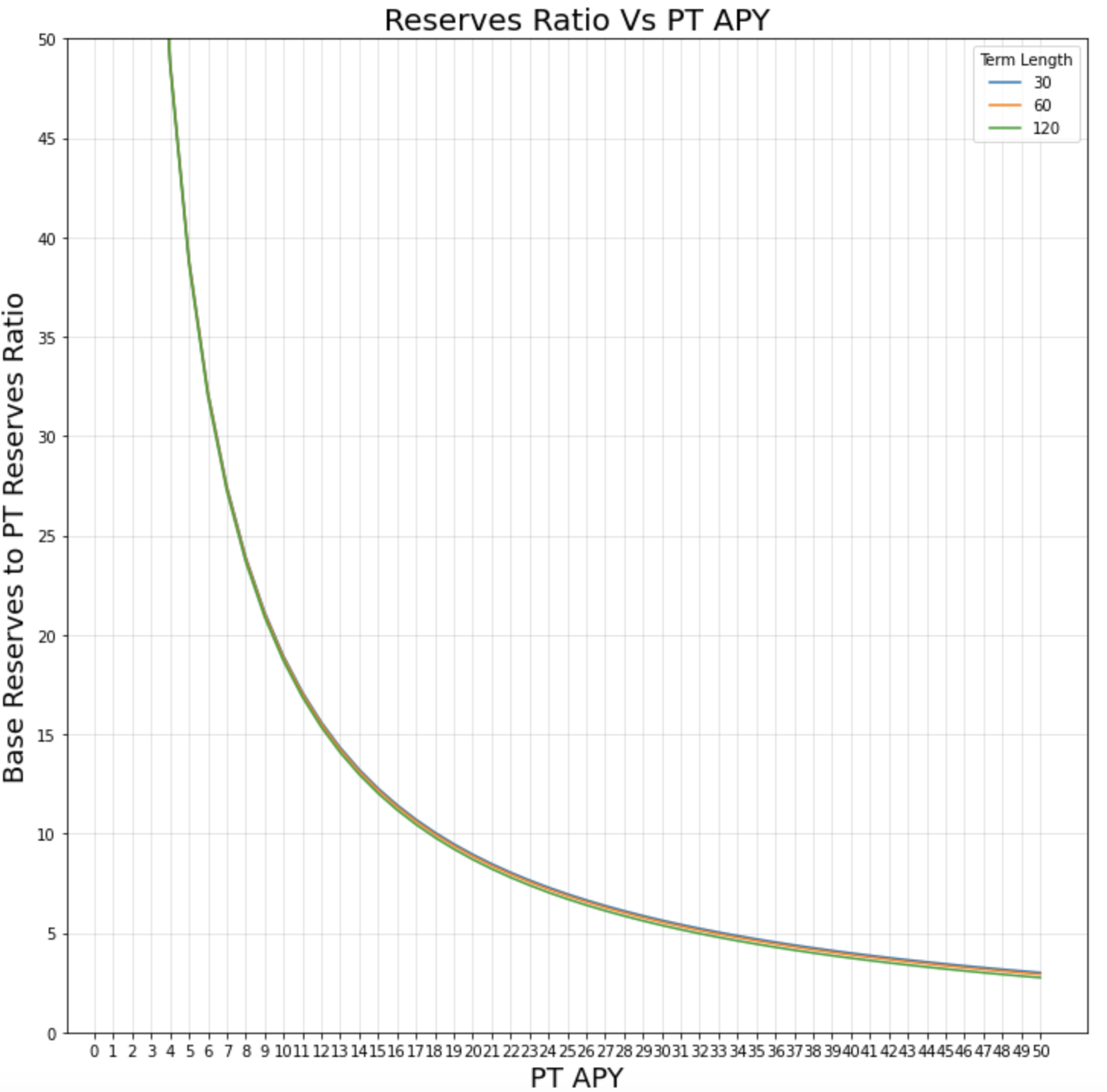
Figure 12
There are two major takeaways from this plot. One, term (or tranche) length does not have a significant affect on the reserve ratios for \(APY_{PT}\)'s < 50%. The second takeaway is that even at a 20% \(APY_{PT}\), for every 1 PT staked, ~9 base asset tokens will be required by LPs. Fortunately, a new parameter can be introduced to the curve to stretch time and reduce the burden on LPs.
Time Stretch
Intuitively, this parameter can be thought of like this:
\begin{aligned} \require{cancel} t &= \frac{term length}{365 \times t_{stretch}} \end{aligned}
where \(t_{stretch}\) is the time stretch parameter. However, since this ONLY applies to the time parameter in the exponent of the pricing invariant (NOT the ratio used to caclulate the APY), the time stretch parameter will be kept separate from the t param for this analysis to avoid confusion. Updating equation (12) to include time stretch:
\begin{aligned} \require{cancel} \frac{x_{r}}{y_r}=\cdot\left(\frac{-2}{\left(1-t\cdot\left(\frac{APY_{PT}}{100}\right)\right)^{\left(\frac{t_{stretch}}{t}\right)}-1}-2\right)\qquad(13) \end{aligned}
Notice that \(t_{stretch}\) only applies to the exponent in the denominator. Now that the time stretch has been parameterized, it can be used to reduce the burden on LPs.
Time Stretch vs Reserve Ratio
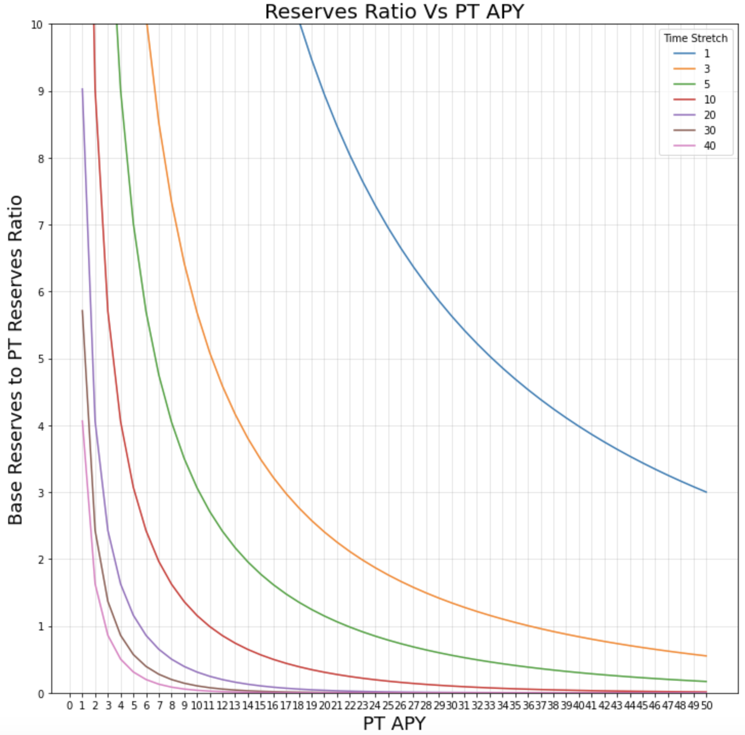
Figure 13
This plot makes it obvious that \(t_{stretch}\) has a significant impact on the ratio of reserves for different \(APY_{PT}\). To understand how this can reduce the burden on LP's, again consider a PT with an APY ~ 20%. As noted before with a time stretch of 1, for every 1 PT staked, ~9 base asset tokens were required by LPs. If the time stretch is changes to 5, then 1 PT staked only needs ~1.2 base assets tokens for a 20% APY. You can see from the plot that the time stretch parameter can also be configured to target 1:1 reserve ratios at lower APYs. This is important for wrapping yield bearing assets like wBTC vaults that might have lower APYs.
On an intuitive level, stretching the time parameter forces the invariant to behave more like it would when near maturity. In other words, since the PTs mature to the value of the base asset, the more t is stretched, the more it behaves like it is near maturity and therefore requires more of an imbalance in reserves to reach a higher APY. This has a beneficial effect when considering the reserve ratios for LPing, but it also impacts the ability to price discover. This is good and bad. Large time stretches will see less slippage; however, a significant change in the APY of the yield bearing asset could incentivize market forces to target a new APY for the PT that it can't realize with too large of a time stretch. It can now be seen how changes in the time stretch parameter impact price discovery.
Time Stretch vs. Price Discovery
In order to determine the impact of the time stretch on price discovery, the max possible trade must be calculated first. To do that, first, recall the pricing invariant from Appendix Section B:
\begin{equation} (out_r-out_q)^{1-\frac{t}{t_{stretch}}}+(in_r+in_q)^{1-\frac{t}{t_{stretch}}}=k\qquad(14) \end{equation}
solving for \(out_q\) is equivalent to the formula for CalculateOutGivenIn (7):
\begin{equation} out_q=out_r-\left(k-\left(in_r+in_q\right)^{\left({1-\frac{t}{t_{stretch}}}\right)}\right)^{\frac{1}{{1-\frac{t}{t_{stretch}}}}}\qquad(15) \end{equation}
Note: Equivalent insights can be developed by using the CalculateInGivenOut (8) variation
Looking at equation (15), it is important to note that:
\begin{equation} k-\left(in_r+in_q\right)^{\left({1-\frac{t}{t_{stretch}}}\right)} \geq 0 \end{equation}
must hold true in order to avoid complex numbers. The boundary can be determined by defining the largest feasible trade by solving for \(in_q\):
\begin{equation} in_q \le k^{\frac{1}{1-\frac{t}{t_{stretch}}}}-in_r \end{equation}
Substituting, \(y_r\) + \(l_{shares}\) for \(in_r\) (as described in the Virtual Reserve Logic, gives:
\begin{equation} Max_{input trade} = k^{\frac{1}{1-\frac{t}{t_{stretch}}}}-(y_r + l_{shares})\qquad(16) \end{equation}
The assumption from earlier that \(l_{shares}\) = \(x_r\) + \(y_r\) still holds so it can also be said that:
\begin{equation} Max_{input trade} = k^{\frac{1}{1-\frac{t}{t_{stretch}}}}-(2y_r + x_{r}) \qquad(16a) \end{equation}
Substituting \(Max_{input\ trade}\) for \(in_q\) and (\(y_r\) + \(l_{shares}\)) for \(in_r\) in equation (15):
\begin{aligned} \require{cancel} out_q&=out_r-\left(k-\left(y_r + l_{shares}+Max_{input trade}\right)^{\left({1-\frac{t}{t_{stretch}}}\right)}\right)^{\frac{1}{{1-\frac{t}{t_{stretch}}}}}\ \newline &=out_r-\left(k-\left(\bcancel{y_r} + \bcancel{l_{shares}}+( k^{\frac{1}{\bcancel{1-\frac{t}{t_{stretch}}}}}-(\bcancel{y_r} + \bcancel{l_{shares}}))\right)^{\bcancel{\left({1-\frac{t}{t_{stretch}}}\right)}}\right)^{\frac{1}{{1-\frac{t}{t_{stretch}}}}}\ \newline &=out_r - \bcancel{(k-k)^{\frac{1}{{1-\frac{t}{t_{stretch}}}}}} \end{aligned}
essentially leaving us with:
\begin{aligned} \require{cancel} out_q&=out_r=x_r \end{aligned}
when \(in_q\) = \(Max_{input\ trade}\). Now that it is known what \(out_q\) is when inputing \(Max_{input\ trade}\), recall that the unit price is the ratio of \(out_q\) to \(in_q\). After substituting what has just been learned, the resulting max unit price is:
\begin{aligned} \require{cancel} Max Unit Price_{PT} &= \frac{x_r}{Max_{input trade}}\qquad(17) \end{aligned}
Solving for \(APY_{PT}\) from equation (9) it is known that:
\begin{aligned} \require{cancel} APY_{PT}=\frac{(1-Unit Price_{PT})}{t}\times100\qquad(18) \end{aligned}
Combining (17) & (18) to get the resulting APY:
\begin{aligned} \require{cancel} Max Resulting APY_{PT}=\frac{\left(1-\frac{x_{r}}{Max_{input trade}}\right)}{t}\times100\qquad(19) \end{aligned}
Equation (19) can now be plotted by sweeping \(APY_{PT}\)'s for several different time stretches and term lengths:
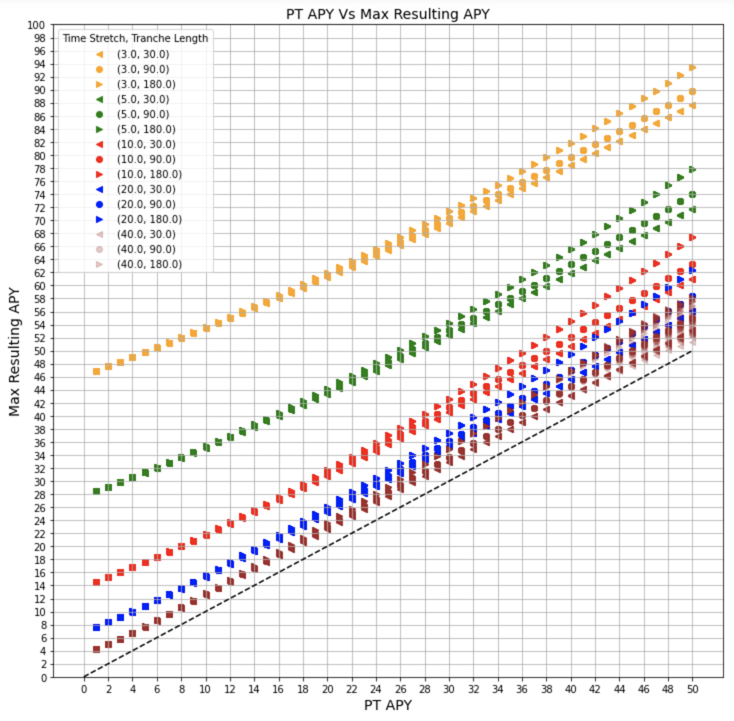
Figure 14
There are several observations to note here. First off, the dash line represents APY = Max Resulting APY. You should never cross below this line. The second observation to note is that, term length starts to have more of an effect on the Max Resulting APY as APY increases. That being said, the difference is < 10% of the Max Resulting APY at the 50% APY input.
Selecting a Time Stretch
The following plot shows what time stretches result in the ratio of the reserves (base/bond) approximately equal to the spot price of the associated APY:
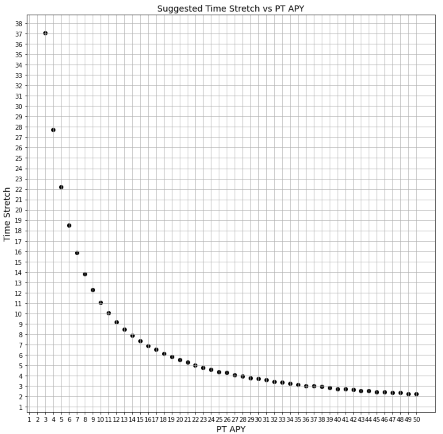
Figure 15a
This plot indicates for example, that for \(APY_{PT}\) = 20%, that \(time\ stretch\) should be approximately 5.5 years. We can stake this one step further and use a curve fitting algorithm to approximate the suggested time stretch for a given \(APY_{PT}\). In order to do this, we first recognize that the curve fitting algorithm will need to approximate coefficients for a function of this form:
\begin{aligned} \frac{a}{b\cdot APY_{PT}}\qquad(20) \end{aligned}
where \(a\) and \(b\) are coefficients calculated by a curve fitting algorithm. Updating (20) with the coefficients that best approximate the values in the previous plot gives us the following equation representing the suggested \(t_{stretch}\) for a given \(APY_{PT}\)
\begin{aligned} t_{stretch}=\frac{3.09396}{0.02789\cdot APY_{PT}}\qquad(21) \end{aligned}
The following plot shows equation (21) overlayed on the previous plot as a green dashed line.
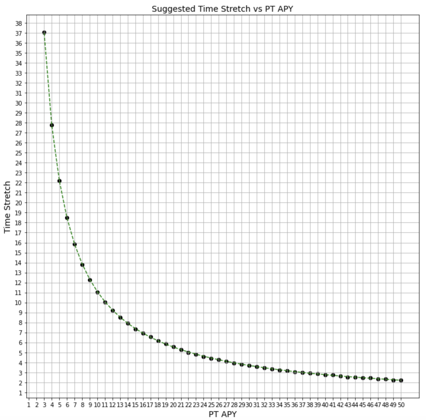
Figure 15b
Visual examination tells us that equation (21) is an excellent approximation for suggested \(time\ stretch\).
C. Compounding and Yield with Element
To understand how the calculations in this writeup are made, please reference the derivation in the next section and analysis.
These tables can be generated with different parameters in this collab.
The compounder incurs risk due to the unknown final value of the accumulated yield, or the average yield gained by the backing yield position. Therefore, the compounder's final APY is determined by how accurate their speculated yield is.
| Yield Position | Yield | Speculated Yield | Term |
|---|---|---|---|
| Yearn STETH | 20% | 15% | 90 days |
| Matured | Input | Liquidity | t-stretch | Gas Used |
|---|---|---|---|---|
| 0 Days | 25 ETH | 5000 ETH | 8 Years | 0.05 ETH |
Expand Table
| PT APY | PT APY after Trade | Total Expenditure | Received at Maturity | APY |
|---|---|---|---|---|
| 8 | 8.89 | 0.608148 | 0.924658 | 211.07 |
| 8.15 | 9.06 | 0.618439 | 0.924658 | 200.81 |
| 8.3 | 9.23 | 0.62873 | 0.924658 | 190.89 |
| 8.45 | 9.39 | 0.639021 | 0.924658 | 181.28 |
| 8.6 | 9.56 | 0.649314 | 0.924658 | 171.98 |
| 8.75 | 9.73 | 0.659607 | 0.924658 | 162.96 |
| 8.9 | 9.89 | 0.669901 | 0.924658 | 154.23 |
| 9.05 | 10.06 | 0.680196 | 0.924658 | 145.76 |
| 9.2 | 10.23 | 0.690492 | 0.924658 | 137.54 |
| 9.35 | 10.4 | 0.700788 | 0.924658 | 129.56 |
| 9.5 | 10.56 | 0.711086 | 0.924658 | 121.81 |
| 9.65 | 10.73 | 0.721385 | 0.924658 | 114.28 |
| 9.8 | 10.9 | 0.731684 | 0.924658 | 106.96 |
| 9.95 | 11.06 | 0.741984 | 0.924658 | 99.85 |
| 10.1 | 11.23 | 0.752286 | 0.924658 | 92.93 |
| 10.25 | 11.4 | 0.762588 | 0.924658 | 86.19 |
| 10.4 | 11.56 | 0.772891 | 0.924658 | 79.64 |
| 10.55 | 11.73 | 0.783196 | 0.924658 | 73.25 |
| 10.7 | 11.9 | 0.793501 | 0.924658 | 67.03 |
| 10.85 | 12.07 | 0.803808 | 0.924658 | 60.97 |
| 11 | 12.23 | 0.814115 | 0.924658 | 55.07 |
| 11.15 | 12.4 | 0.824424 | 0.924658 | 49.31 |
| 11.3 | 12.57 | 0.834734 | 0.924658 | 43.69 |
| 11.45 | 12.74 | 0.845045 | 0.924658 | 38.21 |
| 11.6 | 12.9 | 0.855357 | 0.924658 | 32.86 |
| 11.75 | 13.07 | 0.865671 | 0.924658 | 27.63 |
| 11.9 | 13.24 | 0.875985 | 0.924658 | 22.53 |
| 12.05 | 13.4 | 0.886301 | 0.924658 | 17.55 |
| 12.2 | 13.57 | 0.896618 | 0.924658 | 12.68 |
| 12.35 | 13.74 | 0.906937 | 0.924658 | 7.92 |
| 12.5 | 13.91 | 0.917257 | 0.924658 | 3.27 |
| 12.65 | 14.07 | 0.927578 | 0.924658 | -1.28 |
| 12.8 | 14.24 | 0.9379 | 0.924658 | -5.73 |
| 12.95 | 14.41 | 0.948224 | 0.924658 | -10.08 |
| 13.1 | 14.58 | 0.958549 | 0.924658 | -14.34 |
| 13.25 | 14.74 | 0.968876 | 0.924658 | -18.51 |
| 13.4 | 14.91 | 0.979204 | 0.924658 | -22.59 |
| 13.55 | 15.08 | 0.989533 | 0.924658 | -26.59 |
| 13.7 | 15.25 | 0.999864 | 0.924658 | -30.5 |
| 13.85 | 15.41 | 1.0102 | 0.924658 | -34.34 |
| 14 | 15.58 | 1.02053 | 0.924658 | -38.1 |
| 14.15 | 15.75 | 1.03087 | 0.924658 | -41.78 |
| 14.3 | 15.92 | 1.0412 | 0.924658 | -45.4 |
| 14.45 | 16.09 | 1.05154 | 0.924658 | -48.94 |
| 14.6 | 16.25 | 1.06188 | 0.924658 | -52.41 |
| 14.75 | 16.42 | 1.07223 | 0.924658 | -55.82 |
| 14.9 | 16.59 | 1.08257 | 0.924658 | -59.16 |
Table 5
The above table gives a view of the returns one compound can bring if the estimated accumulated yield, 15% is correct. If the actual average yield at the end of the maturity period is less, then returns decrease. If it is higher, then returns are higher.
The APY column is calculated on the total received, speculated 15%, from the total spent. The total spent includes gas, the discount for selling the PTs, trading fees, and slippage. Although the numbers look quite high, keep in mind the compounder is only receiving that APY on the expenditure, not the total input. Through yield token compounding, each of these small expenditure operations must add up to beat their speculated APY of the actual position. In this case, it must be at 20% for their idle funds to be worth playing the game. Therefore, compounding needs to occur multiple times.
Let us evaluate the same data differently:
| Speculated Yield | Desired Yield |
|---|---|
| 15% | 30% |
Expand Table
| Input | PT APY | PT Price | PT APY after Trade | Spent | Received | Gain | APY |
|---|---|---|---|---|---|---|---|
| 10 | 8.66 | 0.976412 | 9.56629 | 0.295881 | 0.369863 | 0.0739819 | 101.4 |
| 15 | 9.374 | 0.974411 | 10.3776 | 0.443829 | 0.554795 | 0.110966 | 101.4 |
| 20 | 9.719 | 0.973412 | 10.783 | 0.591764 | 0.739726 | 0.147963 | 101.4 |
| 25 | 9.917 | 0.972811 | 11.0266 | 0.739722 | 0.924658 | 0.184935 | 101.39 |
| 30 | 10.041 | 0.972411 | 11.1887 | 0.88766 | 1.10959 | 0.221929 | 101.4 |
| 35 | 10.123 | 0.972126 | 11.3046 | 1.0356 | 1.29452 | 0.258921 | 101.4 |
| 40 | 10.178 | 0.971914 | 11.3906 | 1.18345 | 1.47945 | 0.295998 | 101.43 |
| 45 | 10.217 | 0.971745 | 11.4589 | 1.33147 | 1.66438 | 0.332915 | 101.4 |
| 50 | 10.243 | 0.971612 | 11.5128 | 1.47939 | 1.84932 | 0.369925 | 101.41 |
| 55 | 10.26 | 0.971504 | 11.5567 | 1.62728 | 2.03425 | 0.406963 | 101.42 |
| 60 | 10.271 | 0.971412 | 11.5939 | 1.77527 | 2.21918 | 0.443909 | 101.41 |
| 65 | 10.277 | 0.971334 | 11.6256 | 1.92328 | 2.40411 | 0.480834 | 101.39 |
| 70 | 10.278 | 0.97127 | 11.6515 | 2.07109 | 2.58904 | 0.517955 | 101.42 |
| 75 | 10.277 | 0.971212 | 11.6752 | 2.21912 | 2.77397 | 0.554853 | 101.4 |
| 80 | 10.273 | 0.971162 | 11.6955 | 2.36706 | 2.9589 | 0.591842 | 101.4 |
| 85 | 10.267 | 0.971117 | 11.7135 | 2.51502 | 3.14384 | 0.628812 | 101.4 |
| 90 | 10.259 | 0.971079 | 11.7292 | 2.66291 | 3.32877 | 0.665854 | 101.41 |
| 95 | 10.25 | 0.971043 | 11.7437 | 2.81091 | 3.5137 | 0.702786 | 101.4 |
| 100 | 10.239 | 0.971013 | 11.7558 | 2.95869 | 3.69863 | 0.73994 | 101.43 |
| 105 | 10.228 | 0.970983 | 11.7679 | 3.10676 | 3.88356 | 0.776805 | 101.4 |
| 110 | 10.216 | 0.970956 | 11.7788 | 3.25479 | 4.06849 | 0.8137 | 101.39 |
| 115 | 10.202 | 0.970935 | 11.7873 | 3.40242 | 4.25342 | 0.851002 | 101.44 |
| 120 | 10.189 | 0.970912 | 11.7969 | 3.55059 | 4.43836 | 0.887766 | 101.4 |
| 125 | 10.175 | 0.970891 | 11.8053 | 3.69862 | 4.62329 | 0.924672 | 101.39 |
| 130 | 10.16 | 0.970873 | 11.8124 | 3.84645 | 4.80822 | 0.961767 | 101.41 |
| 135 | 10.145 | 0.970856 | 11.8195 | 3.99444 | 4.99315 | 0.998709 | 101.4 |
| 140 | 10.129 | 0.970842 | 11.8254 | 4.14218 | 5.17808 | 1.03591 | 101.42 |
| 145 | 10.113 | 0.970827 | 11.8311 | 4.29003 | 5.36301 | 1.07299 | 101.43 |
Table 6
The table above optimizes for input values. If multiplying the gain value by 10, then it reaches \(\ge\) to the desired yield of 30% on the input liquidity. Let us evaluate one row:
| Input | PT APY | PT APY after Trade | Spent | Received | Net Gain |
|---|---|---|---|---|---|
| 30 | 10.04 | 11.19 | .89 | 1.12 | .22 |
The compounder has 30 ETH. 30% APY on 30 ETH over 3 months is equal to 2.2 ETH. Multiplying the net gain column by 10 equates to that value. This means 10 compound operations with 30 ETH as input and the PT price at 10.04% returns 30% APY on 30 ETH. Multiplying total spent by 10 means 8.9 ETH is spent during the term period, freeing up 21.1 ETH capital to continue spending on the market or continue compounding, increasing gains further. Since only 8.9 ETH was spent, this means you could see the same compounding gains by using flash loans and only inputting 8.9 ETH in capital.
During this process, the compounder must take their time to wait for the market or price to normalize again. They cannot compound 10 times in a row without incurring significant slippage. As a result, compounding would happen over time. 10 compound operations in this situation put close to 300 ETH liquidity through the AMM, even though the compounder held ~30 ETH to start, and only 8.9 ETH if using flash loans.
Input Thresholds In the table, you'll notice if too little liquidity is used, the PT price needs to be very low for compounding to work, thus making compounding likely unprofitable for lower inputs of capital. This is due to offsetting the expense of gas. At around 30 ETH input, the needed PT APYs begin to converge.
Additionally, if too much liquidity is used, the returns on compounding begin to fall away. This is due to the slippage incurred as an expense. There is an interesting equilibrium to be found here.
In a competitive market, you will notice the PT price peaks at 70 ETH input, then begins dropping off again. It is likely the market will optimize for this input for compounding and for lowering the speculated yield rate.
Increase Speculated Yield
If the desired yield is increased, you see the following results:
| Speculated Yield | Desired Yield |
|---|---|
| 15% | 50% |
Expand Table
| Input | PT APY | PT Price | PT APY after Trade | Spent | Received | Gain | APY |
|---|---|---|---|---|---|---|---|
| 25 | 8.12 | 0.977745 | 9.02576 | 0.616383 | 0.924658 | 0.308275 | 202.83 |
| 30 | 8.249 | 0.977344 | 9.18845 | 0.739693 | 1.10959 | 0.369896 | 202.8 |
| 35 | 8.335 | 0.977059 | 9.30374 | 0.862926 | 1.29452 | 0.431595 | 202.84 |
| 40 | 8.396 | 0.976843 | 9.39148 | 0.986282 | 1.47945 | 0.49317 | 202.79 |
| 45 | 8.438 | 0.976678 | 9.4582 | 1.10947 | 1.66438 | 0.554912 | 202.84 |
| 50 | 8.469 | 0.976544 | 9.51276 | 1.23281 | 1.84932 | 0.616509 | 202.81 |
| 55 | 8.491 | 0.976434 | 9.55734 | 1.35613 | 2.03425 | 0.678114 | 202.79 |
| 60 | 8.506 | 0.976343 | 9.59413 | 1.47941 | 2.21918 | 0.739772 | 202.8 |
| 65 | 8.516 | 0.976266 | 9.62534 | 1.60269 | 2.40411 | 0.801418 | 202.8 |
| 70 | 8.522 | 0.9762 | 9.65207 | 1.72597 | 2.58904 | 0.863068 | 202.8 |
| 75 | 8.525 | 0.976143 | 9.67542 | 1.84929 | 2.77397 | 0.924684 | 202.79 |
| 80 | 8.525 | 0.976094 | 9.69536 | 1.97251 | 2.9589 | 0.986394 | 202.81 |
| 85 | 8.523 | 0.97605 | 9.71303 | 2.09575 | 3.14384 | 1.04809 | 202.82 |
| 90 | 8.52 | 0.976009 | 9.72956 | 2.21916 | 3.32877 | 1.1096 | 202.78 |
| 95 | 8.515 | 0.975974 | 9.74378 | 2.34245 | 3.5137 | 1.17125 | 202.78 |
| 100 | 8.508 | 0.975945 | 9.75567 | 2.46551 | 3.69863 | 1.23312 | 202.84 |
| 105 | 8.501 | 0.975916 | 9.76754 | 2.58886 | 3.88356 | 1.29471 | 202.82 |
| 110 | 8.493 | 0.975889 | 9.77823 | 2.71218 | 4.06849 | 1.35632 | 202.81 |
| 115 | 8.484 | 0.975866 | 9.78772 | 2.83542 | 4.25342 | 1.418 | 202.82 |
| 120 | 8.475 | 0.975843 | 9.79717 | 2.95889 | 4.43836 | 1.47947 | 202.78 |
| 125 | 8.464 | 0.975825 | 9.80426 | 3.08186 | 4.62329 | 1.54143 | 202.84 |
| 130 | 8.454 | 0.975805 | 9.81246 | 3.20537 | 4.80822 | 1.60285 | 202.8 |
| 135 | 8.443 | 0.975788 | 9.81946 | 3.32867 | 4.99315 | 1.66448 | 202.8 |
| 140 | 8.431 | 0.975773 | 9.82523 | 3.45172 | 5.17808 | 1.72636 | 202.84 |
| 145 | 8.42 | 0.975756 | 9.83212 | 3.57532 | 5.36301 | 1.78769 | 202.78 |
Table 7
PT rates are generally lower, therefore in a competitive and efficient market, target APYs should converge to the speculated APY.
Term Periods
Let us evaluate the same situation, but a 30-day term:
| Speculated Yield | Desired Yield |
|---|---|
| 15% | 30% |
Expand Table
| Input | PT APY | PT Price | PT APY after Trade | Spent | Received | Gain | APY |
|---|---|---|---|---|---|---|---|
| 25 | 8.167 | 0.992537 | 9.0795 | 0.246565 | 0.308219 | 0.0616542 | 304.23 |
| 30 | 8.586 | 0.992137 | 9.56635 | 0.295882 | 0.369863 | 0.0739805 | 304.21 |
| 35 | 8.878 | 0.991852 | 9.91347 | 0.345182 | 0.431507 | 0.0863247 | 304.27 |
| 40 | 9.092 | 0.991637 | 10.1748 | 0.394513 | 0.493151 | 0.0986375 | 304.2 |
| 45 | 9.253 | 0.99147 | 10.3777 | 0.443833 | 0.554795 | 0.110962 | 304.18 |
| 50 | 9.377 | 0.991337 | 10.5398 | 0.493144 | 0.616438 | 0.123294 | 304.19 |
| 55 | 9.474 | 0.991228 | 10.6722 | 0.542441 | 0.678082 | 0.135641 | 304.23 |
| 60 | 9.551 | 0.991138 | 10.7824 | 0.591737 | 0.739726 | 0.147989 | 304.28 |
| 65 | 9.613 | 0.991061 | 10.8761 | 0.641052 | 0.80137 | 0.160318 | 304.27 |
| 70 | 9.663 | 0.990995 | 10.9565 | 0.690372 | 0.863014 | 0.172641 | 304.25 |
| 75 | 9.703 | 0.990938 | 11.0257 | 0.739668 | 0.924658 | 0.184989 | 304.29 |
| 80 | 9.736 | 0.990887 | 11.0872 | 0.789022 | 0.986301 | 0.197279 | 304.2 |
| 85 | 9.762 | 0.990843 | 11.1409 | 0.838335 | 1.04795 | 0.20961 | 304.21 |
| 90 | 9.782 | 0.990805 | 11.1878 | 0.88759 | 1.10959 | 0.221999 | 304.31 |
| 95 | 9.799 | 0.990769 | 11.2314 | 0.936971 | 1.17123 | 0.234262 | 304.19 |
| 100 | 9.811 | 0.990738 | 11.2693 | 0.986245 | 1.23288 | 0.246632 | 304.25 |
| 105 | 9.82 | 0.990709 | 11.3039 | 1.03554 | 1.29452 | 0.258983 | 304.28 |
| 110 | 9.827 | 0.990683 | 11.3361 | 1.08491 | 1.35616 | 0.271254 | 304.2 |
| 115 | 9.831 | 0.990659 | 11.365 | 1.13422 | 1.41781 | 0.283585 | 304.2 |
| 120 | 9.833 | 0.990637 | 11.3915 | 1.18355 | 1.47945 | 0.295905 | 304.19 |
| 125 | 9.833 | 0.990617 | 11.4157 | 1.23285 | 1.5411 | 0.308245 | 304.2 |
| 130 | 9.831 | 0.990599 | 11.4376 | 1.2821 | 1.60274 | 0.320635 | 304.27 |
| 135 | 9.828 | 0.990582 | 11.4584 | 1.33141 | 1.66438 | 0.332975 | 304.28 |
| 140 | 9.824 | 0.990566 | 11.4779 | 1.38075 | 1.72603 | 0.34528 | 304.25 |
| 145 | 9.819 | 0.990551 | 11.4963 | 1.43011 | 1.78767 | 0.357565 | 304.2 |
Table 8
Or the same situation, but 60 days into a 90 day term:
Expand Table
| Input | PT APY | PT Price | PT APY after Trade | Spent | Received | Gain | APY |
|---|---|---|---|---|---|---|---|
| 25 | 8.375 | 0.992349 | 9.30864 | 0.862995 | 0.924658 | 0.0616621 | 86.93 |
| 30 | 8.805 | 0.991939 | 9.80774 | 1.0356 | 1.10959 | 0.0739915 | 86.93 |
| 35 | 9.105 | 0.991646 | 10.1638 | 1.20819 | 1.29452 | 0.0863325 | 86.94 |
| 40 | 9.325 | 0.991426 | 10.4319 | 1.38081 | 1.47945 | 0.0986414 | 86.92 |
| 45 | 9.49 | 0.991255 | 10.6394 | 1.5534 | 1.66438 | 0.110987 | 86.93 |
| 50 | 9.618 | 0.991118 | 10.8061 | 1.72601 | 1.84932 | 0.123303 | 86.92 |
| 55 | 9.718 | 0.991007 | 10.9419 | 1.8986 | 2.03425 | 0.135645 | 86.92 |
| 60 | 9.798 | 0.990913 | 11.0556 | 2.07122 | 2.21918 | 0.14796 | 86.91 |
| 65 | 9.862 | 0.990834 | 11.1517 | 2.24382 | 2.40411 | 0.160286 | 86.91 |
| 70 | 9.913 | 0.990767 | 11.2333 | 2.41639 | 2.58904 | 0.172651 | 86.93 |
| 75 | 9.955 | 0.990708 | 11.3049 | 2.58901 | 2.77397 | 0.184961 | 86.92 |
| 80 | 9.989 | 0.990657 | 11.3677 | 2.76164 | 2.9589 | 0.197267 | 86.91 |
| 85 | 10.016 | 0.990612 | 11.4226 | 2.93423 | 3.14384 | 0.209603 | 86.91 |
| 90 | 10.037 | 0.990572 | 11.4708 | 3.10678 | 3.32877 | 0.221983 | 86.93 |
| 95 | 10.054 | 0.990536 | 11.5146 | 3.27938 | 3.5137 | 0.234319 | 86.93 |
| 100 | 10.067 | 0.990504 | 11.5538 | 3.45197 | 3.69863 | 0.246665 | 86.94 |
| 105 | 10.077 | 0.990474 | 11.5896 | 3.62458 | 3.88356 | 0.258981 | 86.93 |
| 110 | 10.084 | 0.990448 | 11.6221 | 3.79718 | 4.06849 | 0.271311 | 86.93 |
| 115 | 10.089 | 0.990423 | 11.6522 | 3.96983 | 4.25342 | 0.28359 | 86.91 |
| 120 | 10.091 | 0.990401 | 11.6789 | 4.1424 | 4.43836 | 0.295959 | 86.93 |
| 125 | 10.092 | 0.99038 | 11.7045 | 4.31506 | 4.62329 | 0.308229 | 86.91 |
| 130 | 10.09 | 0.990362 | 11.7266 | 4.48756 | 4.80822 | 0.320659 | 86.94 |
| 135 | 10.088 | 0.990344 | 11.7486 | 4.66024 | 4.99315 | 0.33291 | 86.91 |
| 140 | 10.084 | 0.990327 | 11.7684 | 4.83283 | 5.17808 | 0.345249 | 86.92 |
| 145 | 10.079 | 0.990312 | 11.7869 | 5.00545 | 5.36301 | 0.357567 | 86.91 |
Table 9
A few observations:
- The range of profitability is shifted up. 30 ETH is no longer profitable to compound with, more funds are necessary.
- Peak PT yield rates that make compounding profitable are slightly lower, but not by much
However, it is proposed that the second point is not true. With 30 days remaining in the 90 day term period or a 30-day term, the market can be more aggressive on its speculated yield. In the case of being 60 days into a 90-day term, more stability is also ensured since YTs have already accumulated most of their yield. In essence, shorter periods allow for a higher speculated yield to be assumed. Let's evaluate both situations and increase the speculated yield:
| Speculated Yield | Desired Yield | Term Period |
|---|---|---|
| 18% | 30% | 30 Days |
Expand Table
| Input | PT APY | PT Price | PT APY after Trade | Spent | Received | Gain | APY |
|---|---|---|---|---|---|---|---|
| 15 | 9.152 | 0.991672 | 10.1327 | 0.184923 | 0.221918 | 0.0369944 | 243.4 |
| 20 | 10.227 | 0.990672 | 11.3493 | 0.246565 | 0.29589 | 0.0493259 | 243.4 |
| 25 | 10.859 | 0.990072 | 12.079 | 0.308198 | 0.369863 | 0.0616646 | 243.43 |
| 30 | 11.27 | 0.989672 | 12.5656 | 0.369837 | 0.443836 | 0.0739985 | 243.44 |
| 35 | 11.555 | 0.989386 | 12.9136 | 0.431488 | 0.517808 | 0.0863201 | 243.4 |
| 40 | 11.761 | 0.989171 | 13.1747 | 0.49314 | 0.591781 | 0.0986404 | 243.36 |
| 45 | 11.914 | 0.989005 | 13.3773 | 0.554778 | 0.665753 | 0.110975 | 243.38 |
| 50 | 12.03 | 0.988872 | 13.5391 | 0.616403 | 0.739726 | 0.123323 | 243.42 |
| 55 | 12.12 | 0.988763 | 13.6723 | 0.678061 | 0.813699 | 0.135637 | 243.38 |
| 60 | 12.19 | 0.988671 | 13.7833 | 0.739722 | 0.887671 | 0.147949 | 243.34 |
| 65 | 12.244 | 0.988595 | 13.8765 | 0.801346 | 0.961644 | 0.160298 | 243.38 |
| 70 | 12.286 | 0.988529 | 13.9564 | 0.862968 | 1.03562 | 0.172649 | 243.41 |
| 75 | 12.319 | 0.988472 | 14.0262 | 0.924629 | 1.10959 | 0.18496 | 243.38 |
| 80 | 12.344 | 0.988422 | 14.0871 | 0.986276 | 1.18356 | 0.197286 | 243.37 |
| 85 | 12.362 | 0.988378 | 14.1401 | 1.04787 | 1.25753 | 0.209662 | 243.43 |
| 90 | 12.376 | 0.988338 | 14.1887 | 1.10957 | 1.33151 | 0.221933 | 243.35 |
| 95 | 12.385 | 0.988303 | 14.2316 | 1.17123 | 1.40548 | 0.234248 | 243.33 |
| 100 | 12.39 | 0.988271 | 14.2699 | 1.23287 | 1.47945 | 0.246586 | 243.35 |
| 105 | 12.392 | 0.988243 | 14.3048 | 1.29452 | 1.55342 | 0.258905 | 243.33 |
| 110 | 12.391 | 0.988217 | 14.3362 | 1.35615 | 1.6274 | 0.27125 | 243.35 |
| 115 | 12.387 | 0.988194 | 14.3641 | 1.4177 | 1.70137 | 0.283668 | 243.44 |
| 120 | 12.382 | 0.988172 | 14.3909 | 1.47937 | 1.77534 | 0.295971 | 243.41 |
| 125 | 12.375 | 0.988152 | 14.4152 | 1.54102 | 1.84932 | 0.308297 | 243.41 |
| 130 | 12.367 | 0.988133 | 14.4384 | 1.60274 | 1.92329 | 0.320549 | 243.33 |
| 135 | 12.357 | 0.988116 | 14.4593 | 1.66438 | 1.99726 | 0.332877 | 243.33 |
| 140 | 12.345 | 0.988101 | 14.4777 | 1.72592 | 2.07123 | 0.345312 | 243.42 |
| 145 | 12.333 | 0.988085 | 14.496 | 1.78761 | 2.14521 | 0.357599 | 243.39 |
Table 9
Or for 60 days into a 90 day term:
Expand Table
| Input | PT APY | PT Price | PT APY after Trade | Spent | Received | Gain | APY |
|---|---|---|---|---|---|---|---|
| 15 | 9.433 | 0.991417 | 10.4421 | 0.628765 | 0.665753 | 0.0369885 | 71.57 |
| 20 | 10.541 | 0.990387 | 11.6954 | 0.838346 | 0.887671 | 0.0493257 | 71.59 |
| 25 | 11.193 | 0.989769 | 12.4474 | 1.04793 | 1.10959 | 0.0616624 | 71.59 |
| 30 | 11.618 | 0.989356 | 12.9498 | 1.25753 | 1.33151 | 0.0739732 | 71.57 |
| 35 | 11.911 | 0.989063 | 13.307 | 1.46709 | 1.55342 | 0.0863313 | 71.59 |
| 40 | 12.124 | 0.988842 | 13.5761 | 1.67669 | 1.77534 | 0.0986491 | 71.58 |
| 45 | 12.282 | 0.98867 | 13.7847 | 1.88626 | 1.99726 | 0.110996 | 71.59 |
| 50 | 12.403 | 0.988532 | 13.9524 | 2.09587 | 2.21918 | 0.123306 | 71.58 |
| 55 | 12.496 | 0.98842 | 14.0892 | 2.30546 | 2.4411 | 0.135635 | 71.58 |
| 60 | 12.568 | 0.988326 | 14.2028 | 2.51503 | 2.66301 | 0.147985 | 71.59 |
| 65 | 12.625 | 0.988247 | 14.2997 | 2.72464 | 2.88493 | 0.160291 | 71.58 |
| 70 | 12.669 | 0.988179 | 14.3822 | 2.93422 | 3.10685 | 0.17263 | 71.58 |
| 75 | 12.703 | 0.98812 | 14.4536 | 3.14379 | 3.32877 | 0.184979 | 71.59 |
| 80 | 12.729 | 0.988069 | 14.516 | 3.35336 | 3.55068 | 0.19733 | 71.6 |
| 85 | 12.749 | 0.988023 | 14.5716 | 3.56297 | 3.7726 | 0.209637 | 71.59 |
| 90 | 12.763 | 0.987983 | 14.6206 | 3.77253 | 3.99452 | 0.221987 | 71.59 |
| 95 | 12.773 | 0.987947 | 14.665 | 3.98215 | 4.21644 | 0.234289 | 71.58 |
| 100 | 12.779 | 0.987914 | 14.7048 | 4.19176 | 4.43836 | 0.2466 | 71.58 |
| 105 | 12.781 | 0.987885 | 14.7401 | 4.4013 | 4.66027 | 0.258977 | 71.59 |
| 110 | 12.781 | 0.987858 | 14.773 | 4.61092 | 4.88219 | 0.271274 | 71.58 |
| 115 | 12.778 | 0.987834 | 14.8025 | 4.82048 | 5.10411 | 0.283628 | 71.59 |
| 120 | 12.773 | 0.987811 | 14.8297 | 5.03006 | 5.32603 | 0.295969 | 71.59 |
| 125 | 12.766 | 0.987791 | 14.8544 | 5.23962 | 5.54795 | 0.30833 | 71.6 |
| 130 | 12.758 | 0.987771 | 14.8781 | 5.44925 | 5.76986 | 0.320615 | 71.58 |
| 135 | 12.748 | 0.987754 | 14.8993 | 5.65881 | 5.99178 | 0.33297 | 71.59 |
| 140 | 12.737 | 0.987738 | 14.9193 | 5.86841 | 6.2137 | 0.345292 | 71.59 |
| 145 | 12.725 | 0.987722 | 14.938 | 6.07802 | 6.43562 | 0.357596 | 71.58 |
Table 10
Peak APY rates are higher and the market will likely find some type of equilibrium between speculated APY and the time remaining.
6 Month Term
| Speculated Yield | Desired Yield | Term Period |
|---|---|---|
| 15% | 30% | 182.5 Days |
Expand Table
| Input | PT APY | PT Price | PT APY after Trade | Spent | Received | Gain | APY |
|---|---|---|---|---|---|---|---|
| 10 | 9.762 | 0.946823 | 10.7832 | 0.591774 | 0.739726 | 0.147952 | 50.7 |
| 15 | 10.107 | 0.944826 | 11.188 | 0.887604 | 1.10959 | 0.221985 | 50.71 |
| 20 | 10.269 | 0.943823 | 11.3914 | 1.18353 | 1.47945 | 0.295919 | 50.7 |
| 25 | 10.357 | 0.943222 | 11.5133 | 1.47944 | 1.84932 | 0.36987 | 50.7 |
| 30 | 10.408 | 0.942822 | 11.5944 | 1.77533 | 2.21918 | 0.443846 | 50.7 |
| 35 | 10.438 | 0.942537 | 11.6523 | 2.07121 | 2.58904 | 0.517828 | 50.7 |
| 40 | 10.455 | 0.942322 | 11.6958 | 2.36711 | 2.9589 | 0.591795 | 50.7 |
| 45 | 10.463 | 0.942157 | 11.7292 | 2.66293 | 3.32877 | 0.665839 | 50.7 |
| 50 | 10.465 | 0.942025 | 11.756 | 2.95875 | 3.69863 | 0.739885 | 50.71 |
| 55 | 10.463 | 0.941915 | 11.7783 | 3.25467 | 4.06849 | 0.813828 | 50.7 |
| 60 | 10.458 | 0.941822 | 11.7972 | 3.55068 | 4.43836 | 0.887675 | 50.69 |
| 65 | 10.45 | 0.941746 | 11.8127 | 3.84653 | 4.80822 | 0.961686 | 50.7 |
| 70 | 10.44 | 0.941681 | 11.8259 | 4.14235 | 5.17808 | 1.03573 | 50.7 |
| 75 | 10.428 | 0.941627 | 11.8367 | 4.43796 | 5.54795 | 1.10998 | 50.72 |
| 80 | 10.416 | 0.941574 | 11.8475 | 4.73409 | 5.91781 | 1.18372 | 50.7 |
| 85 | 10.402 | 0.941532 | 11.856 | 5.02977 | 6.28767 | 1.2579 | 50.71 |
| 90 | 10.388 | 0.941491 | 11.8644 | 5.32584 | 6.65753 | 1.33169 | 50.7 |
| 95 | 10.373 | 0.941455 | 11.8716 | 5.62176 | 7.0274 | 1.40564 | 50.7 |
| 100 | 10.357 | 0.941426 | 11.8776 | 5.91742 | 7.39726 | 1.47984 | 50.71 |
| 105 | 10.341 | 0.941397 | 11.8834 | 6.21335 | 7.76712 | 1.55377 | 50.71 |
| 110 | 10.325 | 0.941368 | 11.8893 | 6.50953 | 8.13699 | 1.62746 | 50.7 |
| 115 | 10.308 | 0.941345 | 11.8939 | 6.80529 | 8.50685 | 1.70156 | 50.7 |
| 120 | 10.291 | 0.941323 | 11.8984 | 7.10124 | 8.87671 | 1.77547 | 50.7 |
| 125 | 10.273 | 0.941307 | 11.9017 | 7.39664 | 9.24658 | 1.84994 | 50.72 |
| 130 | 10.256 | 0.941285 | 11.906 | 7.6929 | 9.61644 | 1.92354 | 50.7 |
| 135 | 10.238 | 0.94127 | 11.9091 | 7.98854 | 9.9863 | 1.99776 | 50.71 |
| 140 | 10.22 | 0.941255 | 11.9121 | 8.28427 | 10.3562 | 2.07189 | 50.71 |
| 145 | 10.202 | 0.941241 | 11.9151 | 8.5801 | 10.726 | 2.14593 | 50.72 |
| 145 | 10.202 | 0.941241 | 11.9151 | 8.5801 | 10.726 | 2.14593 | 50.72 |
Table 11
1 Year Term
| Speculated Yield | Desired Yield | Term Period |
|---|---|---|
| 15% | 30% | 365 Days |
Expand Table
| Input | PT APY | PT Price | PT APY after Trade | Spent | Received | Gain | APY |
|---|---|---|---|---|---|---|---|
| 10 | 10.315 | 0.887644 | 11.3917 | 1.18356 | 1.47945 | 0.295891 | 25.35 |
| 15 | 10.477 | 0.885652 | 11.5936 | 1.77522 | 2.21918 | 0.443956 | 25.36 |
| 20 | 10.548 | 0.884648 | 11.6954 | 2.36704 | 2.9589 | 0.591864 | 25.35 |
| 25 | 10.582 | 0.884046 | 11.7564 | 2.95884 | 3.69863 | 0.73979 | 25.35 |
| 30 | 10.597 | 0.883652 | 11.7964 | 3.55044 | 4.43836 | 0.887916 | 25.36 |
| 35 | 10.602 | 0.883367 | 11.8253 | 4.14216 | 5.17808 | 1.03592 | 25.36 |
| 40 | 10.601 | 0.883148 | 11.8475 | 4.73409 | 5.91781 | 1.18372 | 25.35 |
| 45 | 10.595 | 0.882984 | 11.8641 | 5.32573 | 6.65753 | 1.33181 | 25.35 |
| 50 | 10.586 | 0.882853 | 11.8774 | 5.91733 | 7.39726 | 1.47993 | 25.36 |
| 55 | 10.575 | 0.882746 | 11.8883 | 6.50899 | 8.13699 | 1.62799 | 25.36 |
| 60 | 10.563 | 0.882649 | 11.8981 | 7.10104 | 8.87671 | 1.77567 | 25.35 |
| 65 | 10.549 | 0.882576 | 11.9055 | 7.69257 | 9.61644 | 1.92387 | 25.36 |
| 70 | 10.535 | 0.882503 | 11.9129 | 8.2848 | 10.3562 | 2.07137 | 25.35 |
| 75 | 10.519 | 0.882453 | 11.918 | 8.87602 | 11.0959 | 2.21987 | 25.36 |
| 80 | 10.503 | 0.882404 | 11.923 | 9.4677 | 11.8356 | 2.36792 | 25.36 |
| 85 | 10.487 | 0.882355 | 11.9279 | 10.0598 | 12.5753 | 2.51554 | 25.35 |
| 90 | 10.47 | 0.882319 | 11.9316 | 10.6513 | 13.3151 | 2.66375 | 25.36 |
| 95 | 10.453 | 0.882283 | 11.9352 | 11.2431 | 14.0548 | 2.81166 | 25.36 |
| 100 | 10.436 | 0.882248 | 11.9388 | 11.8352 | 14.7945 | 2.95929 | 25.35 |
| 105 | 10.418 | 0.882225 | 11.9411 | 12.4264 | 15.5342 | 3.10784 | 25.36 |
| 110 | 10.401 | 0.882191 | 11.9445 | 13.019 | 16.274 | 3.25499 | 25.35 |
| 115 | 10.383 | 0.88217 | 11.9467 | 13.6105 | 17.0137 | 3.40319 | 25.35 |
| 120 | 10.365 | 0.882149 | 11.9488 | 14.2021 | 17.7534 | 3.55128 | 25.35 |
| 125 | 10.347 | 0.882129 | 11.9508 | 14.7939 | 18.4932 | 3.69926 | 25.35 |
| 130 | 10.329 | 0.88211 | 11.9528 | 15.3857 | 19.2329 | 3.84713 | 25.35 |
| 135 | 10.311 | 0.882091 | 11.9546 | 15.9777 | 19.9726 | 3.99493 | 25.35 |
| 140 | 10.293 | 0.882074 | 11.9564 | 16.5697 | 20.7123 | 4.14264 | 25.35 |
| 145 | 10.274 | 0.882068 | 11.957 | 17.1601 | 21.4521 | 4.29197 | 25.36 |
Table 12
In both the 1 year and 6-month term, the range of input required for profitability is lowered. Peak PT price for input is lowered as well.
USDC 3 Month
| Yield Position | Yield | Speculated Yield | Term |
|---|---|---|---|
| USDC | 25% | 20% | 90 days |
| Matured | Liquidity | t-stretch | Gas Used |
|---|---|---|---|
| 0 Days | 10,000,000 USDC | 10 Years | 0.06 ETH |
Expand Table
| Input | PT APY | PT Price | PT APY after Trade | Spent | Received | Gain | APY |
|---|---|---|---|---|---|---|---|
| 10000 | 11.739 | 0.968083 | 12.9441 | 419.17 | 493.151 | 73.9804 | 71.58 |
| 20000 | 13.541 | 0.963082 | 14.9721 | 838.351 | 986.301 | 147.95 | 71.57 |
| 30000 | 14.113 | 0.961417 | 15.6477 | 1257.5 | 1479.45 | 221.953 | 71.58 |
| 40000 | 14.378 | 0.960584 | 15.9855 | 1676.65 | 1972.6 | 295.953 | 71.59 |
| 50000 | 14.52 | 0.960085 | 16.1878 | 2095.76 | 2465.75 | 369.997 | 71.6 |
| 60000 | 14.602 | 0.959749 | 16.324 | 2515.05 | 2958.9 | 443.853 | 71.57 |
| 70000 | 14.648 | 0.959512 | 16.4202 | 2934.18 | 3452.05 | 517.875 | 71.58 |
| 80000 | 14.672 | 0.959335 | 16.4921 | 3353.23 | 3945.21 | 591.971 | 71.6 |
| 90000 | 14.682 | 0.959196 | 16.5483 | 3772.36 | 4438.36 | 665.992 | 71.6 |
| 100000 | 14.683 | 0.959082 | 16.5944 | 4191.78 | 4931.51 | 739.729 | 71.57 |
| 110000 | 14.675 | 0.958994 | 16.6303 | 4610.69 | 5424.66 | 813.967 | 71.6 |
| 120000 | 14.663 | 0.958916 | 16.6617 | 5030.02 | 5917.81 | 887.786 | 71.58 |
| 130000 | 14.646 | 0.958854 | 16.6872 | 5449.04 | 6410.96 | 961.918 | 71.59 |
| 140000 | 14.626 | 0.958799 | 16.7092 | 5868.1 | 6904.11 | 1036.01 | 71.6 |
| 150000 | 14.604 | 0.958751 | 16.7288 | 6287.35 | 7397.26 | 1109.91 | 71.59 |
| 160000 | 14.58 | 0.958709 | 16.7459 | 6706.61 | 7890.41 | 1183.8 | 71.59 |
| 170000 | 14.554 | 0.958672 | 16.7606 | 7125.68 | 8383.56 | 1257.88 | 71.59 |
| 180000 | 14.527 | 0.958639 | 16.774 | 7544.9 | 8876.71 | 1331.82 | 71.59 |
| 190000 | 14.499 | 0.95861 | 16.786 | 7964.15 | 9369.86 | 1405.71 | 71.58 |
| 200000 | 14.47 | 0.958583 | 16.7968 | 8383.34 | 9863.01 | 1479.68 | 71.58 |
| 210000 | 14.44 | 0.95856 | 16.8061 | 8802.35 | 10356.2 | 1553.81 | 71.59 |
| 220000 | 14.41 | 0.958538 | 16.8153 | 9221.74 | 10849.3 | 1627.58 | 71.58 |
| 230000 | 14.379 | 0.958518 | 16.8231 | 9640.8 | 11342.5 | 1701.67 | 71.58 |
| 240000 | 14.348 | 0.958499 | 16.8308 | 10060.1 | 11835.6 | 1775.48 | 71.58 |
Table 13
BTC 3 Month
| Yield Position | Yield | Speculated Yield | Term |
|---|---|---|---|
| yWBTC | 20% | 15% | 90 days |
| Matured | Liquidity | t-stretch | Gas Used |
|---|---|---|---|
| 0 Days | 200 BTC | 8 Years | 0.06 ETH |
Expand Table
| Input | PT APY | PT Price | PT APY after Trade | Spent | Received | Gain | APY |
|---|---|---|---|---|---|---|---|
| 0.3 | 8.669 | 0.976412 | 9.56615 | 0.00887633 | 0.0110959 | 0.00221956 | 101.41 |
| 0.4 | 9.21 | 0.974913 | 10.1742 | 0.0118349 | 0.0147945 | 0.00295967 | 101.42 |
| 0.5 | 9.53 | 0.974013 | 10.5392 | 0.0147936 | 0.0184932 | 0.00369959 | 101.42 |
| 0.6 | 9.74 | 0.973411 | 10.7832 | 0.0177532 | 0.0221918 | 0.00443854 | 101.39 |
| 0.7 | 9.886 | 0.972983 | 10.9568 | 0.0207117 | 0.0258904 | 0.0051787 | 101.4 |
| 0.8 | 9.993 | 0.972661 | 11.0874 | 0.0236711 | 0.029589 | 0.00591792 | 101.39 |
| 0.9 | 10.073 | 0.972412 | 11.1884 | 0.026629 | 0.0332877 | 0.00665868 | 101.41 |
| 1 | 10.135 | 0.972212 | 11.2695 | 0.0295878 | 0.0369863 | 0.00739854 | 101.41 |
| 1.1 | 10.184 | 0.972048 | 11.3363 | 0.0325477 | 0.0406849 | 0.00813724 | 101.39 |
| 1.2 | 10.222 | 0.971913 | 11.3909 | 0.0355046 | 0.0443836 | 0.00887893 | 101.42 |
| 1.3 | 10.253 | 0.971797 | 11.4378 | 0.0384638 | 0.0480822 | 0.00961839 | 101.41 |
| 1.4 | 10.278 | 0.971698 | 11.4782 | 0.0414232 | 0.0517808 | 0.0103576 | 101.41 |
| 1.5 | 10.298 | 0.971612 | 11.5129 | 0.0443821 | 0.0554795 | 0.0110973 | 101.41 |
| 1.6 | 10.314 | 0.971537 | 11.5433 | 0.0473407 | 0.0591781 | 0.0118374 | 101.41 |
| 1.7 | 10.327 | 0.97147 | 11.5703 | 0.0503003 | 0.0628767 | 0.0125765 | 101.4 |
| 1.8 | 10.337 | 0.971412 | 11.594 | 0.0532584 | 0.0665753 | 0.013317 | 101.41 |
| 1.9 | 10.345 | 0.971359 | 11.6155 | 0.0562178 | 0.070274 | 0.0140562 | 101.4 |
| 2 | 10.351 | 0.971312 | 11.6347 | 0.0591768 | 0.0739726 | 0.0147958 | 101.4 |
| 2.1 | 10.355 | 0.97127 | 11.6517 | 0.0621337 | 0.0776712 | 0.0155375 | 101.42 |
| 2.2 | 10.358 | 0.97123 | 11.6676 | 0.065093 | 0.0813699 | 0.0162769 | 101.41 |
| 2.3 | 10.36 | 0.971194 | 11.6824 | 0.0680537 | 0.0850685 | 0.0170148 | 101.4 |
| 2.4 | 10.36 | 0.971163 | 11.6949 | 0.0710084 | 0.0887671 | 0.0177588 | 101.43 |
| 2.5 | 10.36 | 0.971132 | 11.7074 | 0.0739692 | 0.0924658 | 0.0184965 | 101.41 |
| 2.6 | 10.359 | 0.971104 | 11.7188 | 0.076929 | 0.0961644 | 0.0192354 | 101.41 |
| 2.7 | 10.357 | 0.971079 | 11.7291 | 0.0798869 | 0.099863 | 0.0199761 | 101.41 |
| 2.8 | 10.354 | 0.971056 | 11.7382 | 0.0828419 | 0.103562 | 0.0207198 | 101.43 |
| 2.9 | 10.351 | 0.971034 | 11.7473 | 0.0858014 | 0.10726 | 0.0214589 | 101.43 |
| 3 | 10.348 | 0.971012 | 11.7564 | 0.0887653 | 0.110959 | 0.0221936 | 101.4 |
| 3.1 | 10.344 | 0.970992 | 11.7644 | 0.091725 | 0.114658 | 0.0229325 | 101.39 |
| 3.2 | 10.339 | 0.970975 | 11.7712 | 0.0946795 | 0.118356 | 0.0236767 | 101.42 |
| 3.3 | 10.334 | 0.970958 | 11.778 | 0.0976373 | 0.122055 | 0.0244175 | 101.42 |
| 3.4 | 10.329 | 0.970942 | 11.7848 | 0.100598 | 0.125753 | 0.0251551 | 101.41 |
| 3.5 | 10.323 | 0.970928 | 11.7904 | 0.103553 | 0.129452 | 0.0258993 | 101.43 |
| 3.6 | 10.318 | 0.970911 | 11.7972 | 0.10652 | 0.133151 | 0.0266307 | 101.39 |
| 3.7 | 10.311 | 0.9709 | 11.8016 | 0.109469 | 0.136849 | 0.0273798 | 101.44 |
| 3.8 | 10.305 | 0.970886 | 11.8072 | 0.112432 | 0.140548 | 0.0281161 | 101.42 |
| 3.9 | 10.299 | 0.970873 | 11.8128 | 0.115397 | 0.144247 | 0.0288498 | 101.39 |
| 4 | 10.292 | 0.970862 | 11.8172 | 0.118353 | 0.147945 | 0.0295922 | 101.4 |
| 4.1 | 10.285 | 0.970851 | 11.8216 | 0.121311 | 0.151644 | 0.0303326 | 101.4 |
| 4.2 | 10.278 | 0.97084 | 11.826 | 0.124271 | 0.155342 | 0.031071 | 101.4 |
| 4.3 | 10.27 | 0.970832 | 11.8292 | 0.127221 | 0.159041 | 0.0318197 | 101.43 |
| 4.4 | 10.263 | 0.970822 | 11.8335 | 0.130185 | 0.16274 | 0.0325544 | 101.41 |
| 4.5 | 10.255 | 0.970814 | 11.8367 | 0.133138 | 0.166438 | 0.0333001 | 101.44 |
| 4.6 | 10.248 | 0.970803 | 11.841 | 0.136106 | 0.170137 | 0.0340312 | 101.4 |
| 4.7 | 10.24 | 0.970795 | 11.8441 | 0.139062 | 0.173836 | 0.0347739 | 101.41 |
| 4.8 | 10.232 | 0.970788 | 11.8472 | 0.142019 | 0.177534 | 0.0355153 | 101.42 |
| 4.9 | 10.224 | 0.97078 | 11.8503 | 0.144978 | 0.181233 | 0.0362553 | 101.42 |
Table 14
Yield Token Discussion
In all the above scenarios, something fascinating is discovered. YTs become a very lucrative purchase. Let us evaluate a row from the BTC 3 month term:
| Input | PT APY | PT APY after Trade | Spent | Received | Gain |
|---|---|---|---|---|---|
| 1 | 10.135 | 11.2695 | 0.0295878 | 0.0369863 | 0.00739854 |
If the YT is priced at greater than the "Spent" value, then its price will be immediately pushed back down. For the following illustration, let us assume the YT is now selling for 0.031 BTC.
- Mint 1 PT and 1 YT, total input 1 BTC
- Sell PT (1 - "Spent" = 0.971 BTC including gas fees)
- Sell YT (0.031)
- 0.971 + 0.031 = 0.001 BTC profit
Someone will be able to mint and immediately sell both the PT and YT for profit. However, let us look at that table row again with a new column added to it:
| Input | PT APY | PT APY after Trade | Spent | Received | Gain | APY |
|---|---|---|---|---|---|---|
| 1 | 10.135 | 11.2695 | 0.0295878 | 0.0369863 | 0.00739854 | 101.41 |
If the YT is priced at 0.03 BTC, but returns 0.037 BTC at the end of 3 months, purchasing the YT will give a 93.59% APY. However, by default, YT purchases will not be able to support the same amount of liquidity as PTs. 1 BTC PT matures to 1 BTC. 1 BTC PT, in this case, matures to 0.037 BTC. In an AMM, this means PTs have much more backing liquidity than PTs. The market will find equilibrium, but purchasing and selling PTs can be done with large amounts of liquidity. PTs do not have the same liquidity. Yield Token Compounding, therefore, supports high liquidity. Purchasing YTs will likely be smaller quantities. The market will find equilibrium somewhere.
What can be predicted? Mainly that equilibrium will be found and it is yet to be seen how the market will react exactly. Purchasing YTs and yield token compounding are both highly profitable endeavors.
Further Discussion
In all the examples shared, if the final yield is higher than the speculated yield, then yield token compounding becomes significantly more profitable than the targeted yield.
Initial Pool Parameterization
To parameterize the initial pools, you set the t-stretch to match the optimal input and associated PT APY for yield token compounding when the speculated yield is set to 75% of the yield position's APY and the desired yield is set to 150% of the position's APY. Next, take the calculated PT APY and set our t-stretch in accordance with the analysis in Appendix B. This is called the 75/150% rule.
D. Yield Token Compounding Formulation
Calculate the max market \(APY_{PT}\) that allows me to hit \(APY_{target}\) after \(N\) compounds assuming \(APY_{speculated}\) for a given \(Token_{input}\) and \(term\ length\)
Begin by defining the target number of accrued tokens needed after the \(term\) has expired in order to hit the \(APY_{target}\):
\begin{aligned} \require{cancel}\ Token_{target} &= Token_{input} \times \frac{APY_{target}}{100} \times t \end{aligned}
where \(t\) is defined as:
\begin{aligned} \require{cancel} t &= \frac{term length}{365} \end{aligned}
Next, it is defined how to quantify the net tokens earned over a \(term\). To do this, the tokens earned needs to be quantified:
\begin{aligned} \require{cancel}\ Token_{earned} &= Token_{input} \times \frac{APY_{speculated}}{100} \times t \end{aligned}
and the tokens spent in a \(term\) for a single compound:
\begin{aligned} \require{cancel} Token_{spent} &= Token_{input} - Unit Price \times Token_{input} + Fee_{gas} \end{aligned}
Taking the difference between the \(Token_{earned}\) and \(Token_{spent}\) gives us the net tokens earned:
\begin{aligned} \require{cancel} Token_{net} &= Token_{earned}-Token_{spent} \end{aligned}
and the following inequality that compares the net number of tokens earned after N compounds and some time period \(t\):
\begin{aligned} \require{cancel} Token_{net} \times N \ge Token_{target} \qquad(22) \end{aligned}
Equation (22) in expanded form:
\begin{aligned} \require{cancel} \left((Token_{input} \times \frac{APY_{speculated}}{100} \times t) - ( Token_{input} - Unit Price \times Token_{input} + Fee_{gas})\right)\times N \ge Token_{input} \times\frac{APY_{target}}{100} \times t \end{aligned}
solving for \(Unit\ Price\):
\begin{aligned} \require{cancel} Unit Price \ge 1- \frac{APY_{speculated}}{100} \times t - \frac{APY_{target}}{100 \times N} \times t - \frac{Fee_{gas}}{Token_{input}} \end{aligned}
allows us can calculate the minimum PT market price (after slippage) needed to hit the \(APY_{target}\):
\begin{aligned} \require{cancel} Unit Price_{min} = 1- \frac{APY_{speculated}}{100} \times t - \frac{APY_{target}}{100 \times N} \times t - \frac{Fee_{gas}}{Token_{input}} \qquad(23) \end{aligned}
Recall that \(APY_{PT}\) can be defined as:
\begin{aligned} \require{cancel} APY_{PT}=\frac{(1-Unit Price_{PT})}{t} \times 100 \end{aligned}
and combined with (23) the max market \(APY_{target}\) is:
\begin{aligned} \require{cancel} APY_{PT} = \frac{\frac{APY_{speculated}}{100} \times t - \frac{APY_{target}}{100 \times N} \times t - \frac{Fee_{gas}}{Token_{input}}}{100} \times t \qquad(24) \end{aligned}
Calculate the number of Principal Tokens (PTs) and Yield Tokens (YTs) you are left with after N compounds:
\begin{aligned} Number of PTs = P\cdot\left(1-R\right)^{N}\qquad(25) \end{aligned}
where \(P\) is the initial principal amount deposited and \(R\) is the market rate of the \(PT\). The \(Number\ of\ YTs\) can represented by the following summation:
\begin{aligned} S&=P\cdot \sum_{i=0}^{N}\left(1-R\right)^{i} \qquad(26) \end{aligned}
The summation in equation (26) can be expanded as follows:
\begin{aligned} S&=P\cdot\left(1+\left(1-R\right)^{1}+\left(1-R\right)^{2}+...+\left(1-R\right)^{N}\right)\qquad(27) \end{aligned}
Multiplying both sides of equation (27) by \((1-R)\) gives us:
\begin{aligned} (1-R)\cdot S&=P\cdot\left(\left(1-R\right)^{1}+\left(1-R\right)^{2}+...+\left(1-R\right)^{N}+\left(1-R\right)^{N+1}\right)\qquad(28) \end{aligned}
Subtracting (28) from (27), simplifying and solving for \(S\):
\begin{aligned} \require{cancel} S - S \cdot (1-R)&=P\cdot\left(\left(1+\left(1-R\right)^{1}+\left(1-R\right)^{2}+...+\left(1-R\right)^{N}\right) - \left(\left(1-R\right)^{1}+\left(1-R\right)^{2}+...+\left(1-R\right)^{N}+\left(1-R\right)^{N+1}\right)\right)\ \newline \bcancel{S - S} + R\cdot S &= P\cdot\left(\left(1+\bcancel{\left(1-R\right)^{1}}+\bcancel{\left(1-R\right)^{2}}+...+\bcancel{\left(1-R\right)^{N}}\right) - \left(\bcancel{\left(1-R\right)^{1}}+\bcancel{\left(1-R\right)^{2}}+...+\bcancel{\left(1-R\right)^{N}}+\left(1-R\right)^{N+1}\right)\right)\ \newline S&=\frac{P\cdot\left(1-\left(1-R\right)^{N+1}\right)}{R} \end{aligned}
Now it can be said that:
\begin{aligned} Number of YTs &=\frac{P\cdot\left(1-\left(1-R\right)^{N+1}\right)}{R}\qquad(29) \end{aligned}
E. Initializing the Convergent Curve Pool Price
The convergent curve pool price is initialized in two steps. First, the pool must be seeded with initial liquidity in the form of the base asset. Second, a trade is executed to initialize the price to match the initial \(APY_{PT}\). If you recall equation (18) that relates \(APY_{PT}\) to \(Unit\ Price_{PT}\):
\begin{aligned} \require{cancel} APY_{PT}=\frac{(1-Unit Price_{PT})}{t}\times100 \end{aligned}
Additionally, from equation (10), we know that \(Unit\ Price_{PT}\) is defined in terms of \(x_r\), \(y_r\), \(l_{shares}\) and \(t\):
\begin{aligned} \require{cancel} Unit Price_{PT} &= \left(\frac{y_{r}+l_{shares}}{x_{r}}\right)^{-t} \end{aligned}
Combining (18) & (10) gives us:
\begin{aligned} \require{cancel} APY_{PT}=\frac{\left(1-\left(\frac{y_{r}+l_{shares}}{x_{r}}\right)^{-\frac{t}{t_{stretch}}}\right)}{t}\times100\qquad(30) \end{aligned}
It is important to note that since only the initial deposit of the base token has been made, we know that \(y_r\)=0 and \(x_r\) = \(l_{shares}\) resulting in the initial \(Unit\ Price_{PT}\) = 1. As a result, we simplify (30) as follows:
\begin{aligned} \require{cancel} APY_{PT}=\frac{\left(1-\left(\frac{x_{r}}{x_{r}}\right)^{-\frac{t}{t_{stretch}}}\right)}{t}\times100\qquad(31) \end{aligned}
Remember, the goal is to calculate the trade needed to initialize the pool to \(APY_{PT}\). This essentially means that we need to solve for \(\delta\)y in this equation:
\begin{aligned} \require{cancel} APY_{PT}=\frac{\left(1-\left(\frac{x_{r}+\delta y}{x_{r}-\delta y}\right)^{-\frac{t}{t_{stretch}}}\right)}{t}\times100 \end{aligned}
We use \(\delta\)y to represent the amount of the PT entering the pool AND the amount of the base token exiting the pool. We do this because \(Unit\ Price_{PT}\) = 1 and we are disregarding slippage for simplicity.
\begin{aligned} \require{cancel} \frac{1-\left(\frac{x_{r}+\delta y}{x_{r}-\delta y}\right)^{-\frac{t}{t_{stretch}}}}{t}&=\frac{APY_{PT}}{100}\ \newline \left(\frac{x_{r}+\delta y}{x_{r}-\delta y}\right)^{-\frac{t}{t_{stretch}}}&=1-\frac{APY_{PT}}{100}\times t\ \newline \frac{x_{r}+\delta y}{x_{r}-\delta y}&=\left(1-\frac{APY_{PT}}{100}\times t\right)^{-\frac{t_{stretch}}{t}}\ \newline x_{r}+\delta y&=\left(1-\frac{APY_{PT}}{100}\times t\right)^{-\frac{t_{stretch}}{t}}(x_{r}-\delta y)\ \newline x_{r}+\delta y&=x_{r}\left(1-\frac{APY_{PT}}{100}\times t\right)^{-\frac{t_{stretch}}{t}}-\delta y\left(1-\frac{APY_{PT}}{100}\times t\right)^{-\frac{t_{stretch}}{t}}\ \end{aligned}
Solving for \(\delta y\), gives the amount of PT to trade into the pool to ensure that it is initialized to \(APY_{PT}\): \begin{aligned} \require{cancel} \delta y&=\frac{x_{r}\left(\left(1-\frac{APY_{PT}}{100}\times t\right)^{-\frac{t_{stretch}}{t}}-1\right)}{\left(1+\left(1-\frac{APY_{PT}}{100}\times t\right)^{-\frac{t_{stretch}}{t}}\right)}\qquad(32) \end{aligned}
Note: this procedure does not account for slippage; however, it is accurate enough for this initializing trade.